Introduction to Data Analysis with Python
Erick Martins Ratamero
Research Fellow
- These slides: http://tiny.cc/camdupython2 (redirects to https://erickmartins.github.io/DataAnalysisPython.html)
- Tidy data
- Some relevant libraries
- String manipulation
- File input/output
- Plotting
- If we have time: introduction to pandas and numpy
"Happy families are all alike; every unhappy family is unhappy in its own way"
Leo Tolstoy
We will discuss a standardised way to link the structure of a dataset to its semantics.
(i.e. we will relate the physical layout of data to its meaning in a predictable way.)
import pandas as pd
test = pd.read_csv("test.csv")
test
      name condition1 condition2
 1   Alice         NA          8
 2     Bob          4          2
 3   Carol          6          9
import pandas as pd
test2 = pd.read_csv("test2.csv")
test2
   condition      Alice      Bob        Carol
 1         1         NA        4            6
 2         2          8        2            9
Data is the same, but layout is different - no easy way of knowing it is the same data!
A dataset is a collection of values.
A value belongs to a variable and an observation.
A variable contains all values that measure the same attribute (height, duration, frequency).
An observation contains all values measured on the same "experiment".
import pandas as pd
test_tidy = pd.read_csv("test_tidy.csv")
test_tidy
      name condition       n
 1   Alice         1      NA
 2   Alice         2       8
 3     Bob         1       4
 4     Bob         2       2
 5   Carol         1       6
 6   Carol         2       9
Tidy data depends on your experimental design.
Each variable should be a column.
Each observation should be a row.
Each type of observation (demographic, medical, meteorological, etc.) should be a table.
- Column headers as values instead of variable names
- Multiple variables in the same column
- Variables in rows and columns
- Multiple types of obervations in the same table
- Same type of observation in different tables
    religion `<$10k` `$10-20k` `$20-30k` `$30-40k` `$40-50k` `$50-75k`
  1 Agnostic      27        34        60        81        76       137
  2 Atheist       12        27        37        52        35        70
  3 Buddhist      27        21        30        34        33        58
  4 Catholic     418       617       732       670       638      1116
  5 Don’t k…      15        14        15        11        10        35
  6 Evangel…     575       869      1064       982       881      1486
  7 Hindu          1         9         7         9        11        34
  8 Histori…     228       244       236       238       197       223
  9 Jehovah…      20        27        24        24        21        30
 10 Jewish        19        19        25        25        30        95
    iso2   year   m04  m514  m014 m1524 m2534 m3544 m4554 m5564   m65    mu
  1 AD     1989    NA    NA    NA    NA    NA    NA    NA    NA    NA    NA
  2 AD     1990    NA    NA    NA    NA    NA    NA    NA    NA    NA    NA
  3 AD     1991    NA    NA    NA    NA    NA    NA    NA    NA    NA    NA
  4 AD     1992    NA    NA    NA    NA    NA    NA    NA    NA    NA    NA
  5 AD     1993    NA    NA    NA    NA    NA    NA    NA    NA    NA    NA
  6 AD     1994    NA    NA    NA    NA    NA    NA    NA    NA    NA    NA
  7 AD     1996    NA    NA     0     0     0     4     1     0     0    NA
  8 AD     1997    NA    NA     0     0     1     2     2     1     6    NA
  9 AD     1998    NA    NA     0     0     0     1     0     0     0    NA
 10 AD     1999    NA    NA     0     0     0     1     1     0     0    NA
    id     year month element    d1    d2    d3    d4    d5    d6    d7
  1 MX17…  2010     1 tmax       NA  NA    NA      NA  NA      NA    NA
  2 MX17…  2010     1 tmin       NA  NA    NA      NA  NA      NA    NA
  3 MX17…  2010     2 tmax       NA  27.3  24.1    NA  NA      NA    NA
  4 MX17…  2010     2 tmin       NA  14.4  14.4    NA  NA      NA    NA
  5 MX17…  2010     3 tmax       NA  NA    NA      NA  32.1    NA    NA
  6 MX17…  2010     3 tmin       NA  NA    NA      NA  14.2    NA    NA
  7 MX17…  2010     4 tmax       NA  NA    NA      NA  NA      NA    NA
  8 MX17…  2010     4 tmin       NA  NA    NA      NA  NA      NA    NA
  9 MX17…  2010     5 tmax       NA  NA    NA      NA  NA      NA    NA
 10 MX17…  2010     5 tmin       NA  NA    NA      NA  NA      NA    NA
- numpy: NUMerical PYthon. Has multidimensional arrays, basic linear algebra, Fourier transforms, random number generation...
- scipy: SCIentific PYthon. Higher-level science and engineering modules (optimization, e.g.).
- matplotlib: Plotting library. Histograms, line plots, heat plots...
- pandas: Structured data manipulation and operations. Data scientists love this one.
- seaborn: Also does plotting, but it looks nice compared to matplotlib.
- os: Opeating system stuff and file operations.
We've talked a little bit about strings before.
What if we want a string containing a quote?
string = 'That is Erick's presentationFix: use double quotes!
string = "That is Erick's presentation"What if we need double quotes in the string?
\'Single quote\"Double quote\tTab\nNew line (or line break)\\backslash
>>> print("Hello there!\nHow are you?\nI\'m doing fine.")
Hello there!
How are you?
I'm doing fine.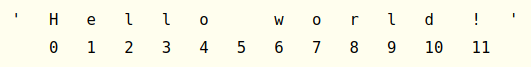
Strings use indexing the same way lists do. It's just a list of characters! The space and exclamation points count, so 'Hello world!' has 12 characters (from 0 to 11).
>>> test = 'Hello world!'
>>> test[0]
'H'
>>> test[4]
'o'
>>> test[-1]
'!'
>>> test[0:5]
'Hello'
>>> test[:5]
'Hello'
>>> test[6:]
'world!'
The in and not in operators work for strings as well as lists (have I mentioned that strings are just lists of characters?). It will return True or False.
>>> 'Hello' in 'Hello world!'
True
>>> 'Hello' in 'Hello'
True
>>> 'HELLO' in 'Hello world!'
False
>>> '' in 'test'
True
>>> 'cats' not in 'cats and dogs'
False
The startswith() and endswith() methods return True if the string they are called on begins or (respectively) ends with the string passed to the method.
>>> 'Hello world!'.startswith('Hello')
True
>>> 'Hello world!'.endswith('world!')
True
>>> 'abc123'.startswith('abcdef')
False
>>> 'abc123'.endswith('12')
False
>>> 'Hello world!'.startswith('Hello world!')
True
>>> 'Hello world!'.endswith('Hello world!')
True
The join() and split() do what you expect them to do. split() can take a string argument and will split the string upon the occurrence of this argument. It is especially useful when dealing with CSV files, as we will see later.
>>> ', '.join(['cats', 'rats', 'bats'])
'cats, rats, bats'
>>> ' '.join(['My', 'name', 'is', 'Simon'])
'My name is Simon'
>>> 'ABC'.join(['My', 'name', 'is', 'Simon'])
'MyABCnameABCisABCSimon'
>>> 'My name is Simon'.split()
['My', 'name', 'is', 'Simon']
>>> 'MyABCnameABCisABCSimon'.split('ABC')
['My', 'name', 'is', 'Simon']
>>> 'My name is Simon'.split('m')
['My na', 'e is Si', 'on']
We can use strip() and its friends to remove whitespace characters (space, tab, newline) from the ends of a string. It returns a new string without the whitespaces.
>>> spam = '    Hello World     '
>>> spam.strip()
'Hello World'
>>> spam.lstrip()
'Hello World     '
>>> spam.rstrip()
'    Hello World'
Alternatively, you can tell strip() which characters you want to remove.
>>> spam = 'SpamSpamBaconSpamEggsSpamSpam'
>>> spam.strip('ampS')
'BaconSpamEggs'
- Write a Python program to calculate the length of a string.
- Write a Python program to add 'ing' at the end of a given string (length should be at least 3). If the given string already ends with 'ing' then add 'ly' instead. If the string length of the given string is less than 3, leave it unchanged. ('abc' returns 'abcing', 'string' returns 'stringly', etc etc)
Sample solution 1
def string_length(str1):
    count = 0
    for char in str1:
        count += 1
    return count
print(string_length('test'))
Sample solution 2
def add_string(str1):
  length = len(str1)

  if length > 2:
    if str1[-3:] == 'ing':
      str1 += 'ly'
    else:
      str1 += 'ing'

  return str1
print(add_string('ab'))
print(add_string('abc'))
print(add_string('string'))- Every file contains three key pieces of information: path, filename and extension.
- path: indicates in which folder the file exists. Can be something like
C:\Users\User1\Desktop\on Windows and/home/User1/Desktopon Mac/Linux. - filename: the actual name of the file. Can be essentially anything you want except for some special characters.
- extension: indicates the file type. Common extensions are
.doc, .xls, .txtand so on. They are often hidden in Windows.
As you can see from the examples, Windows has a different way of indicating folders compared to Mac/Linux, including some weird backslashes.
If you want your code to run in any system, it needs to be aware of which system it is! os.path.join() is your best friend.
>>> import os
>>> os.path.join('usr', 'bin', 'spam')
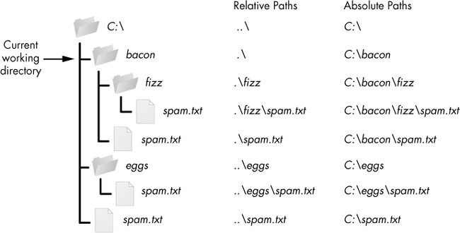
'usr\\bin\\spam'Every program has a current working directory - every path that doesn't start with the root folder (C:\ on Windows, / on Mac/Linux) is presumed to be inside the current working directory.
>>> import os
>>> os.getcwd()
'C:\\Python34'
>>> os.chdir('C:\\Windows\\System32')
>>> os.getcwd()
'C:\\Windows\\System32'
File paths can be absolute (starts with root directory) or relative (from the current working directory).
Some additional os functions that can be useful:
>>> os.path.abspath('.\\Scripts')
'C:\\Python34\\Scripts'
>>> os.path.relpath('C:\\Windows', 'C:\\spam\\eggs')
'..\\..\\Windows'
>>> os.getcwd()
'C:\\Python34'
>>> path = 'C:\\Windows\\System32\\calc.exe'
>>> os.path.basename(path)
'calc.exe'
>>> os.path.dirname(path)
'C:\\Windows\\System32'
>>> os.path.split(path)
('C:\\Windows\\System32', 'calc.exe')
>>> os.path.exists('C:\\Windows')
True
>>> os.path.exists('C:\\some_made_up_folder')
False
>>> os.path.isdir('C:\\Windows\\System32')
True
>>> os.path.isfile('C:\\Windows\\System32')
False
>>> os.path.isdir('C:\\Windows\\System32\\calc.exe')
False
>>> os.path.isfile('C:\\Windows\\System32\\calc.exe')
True
For finding everything that is inside a folder, use os.listdir(path):
>>> os.listdir('C:\\Windows\\System32')
['0409', '12520437.cpx', '12520850.cpx', '5U877.ax', 'aaclient.dll',
--snip--
'xwtpdui.dll', 'xwtpw32.dll', 'zh-CN', 'zh-HK', 'zh-TW', 'zipfldr.dll']
If you want to recursively go into every subfolder, you will need something like this:
>>> import os
>>> path = '/home/erick/Desktop'
>>> for root,dirs,files in os.walk('.'):
...     print("current directory is "+root)
...     print("immediate subdirectories are "+' '.join(dirs))
...     print("files in this subfolder are "+' '.join(files))
...
current directory is .
immediate subdirectories are js img-ia css .git plugin test img img-py lib material
files in this subfolder are test.md bower.json handout.png DataAnalysisPython.html package.json LICENSE ImageAnalysisWithFiji.html CONTRIBUTING.md index.html README.md Gruntfile.js README_REVEAL.md IntroPython.html ImageAnalysis.html
current directory is ./js
(...)
To read or write files, you first need to open them. Try saving the file hello.txt file on your home folder and then opening it:
>>> helloFile = open('C:\\Users\\your_home_folder\\hello.txt')Or if you're Mac/Linux
>>> helloFile = open('/Users/your_home_folder/hello.txt')This will open the file in read-only mode. If you want to open the file in write mode:
>>> helloFile = open('/Users/your_home_folder/hello.txt', 'w')Two ways of reading the contents of a file (try it yourself with the sonnet29.txt file):
>>> f = open('/Users/your_home_folder/sonnet29.txt')
>>> f.read()
"When, in disgrace with fortune and men's eyes,\nI all alone beweep my outcast state,\nAnd trouble deaf heaven with my bootless cries,\nAnd look upon myself and curse my fate,"
>>> f2 = open('material/sonnet29.txt')
>>> f2.readlines()
["When, in disgrace with fortune and men's eyes,\n", 'I all alone beweep my outcast state,\n', 'And trouble deaf heaven with my bootless cries,\n', 'And look upon myself and curse my fate,']
Now let's try writing to a file. Remember: we need to use 'w' when opening it. After that, we just need to use the write method:
>>> myFile = open('test.txt', 'w')
>>> myFile.write('Hello world!\n')
>>> myFile.close()
>>> myFile = open('test.txt', 'a')
>>> myFile.write('This is a nice extra message!')
>>> myFile.close()
>>> myFile = open('test.txt')
>>> content = myFile.read()
>>> myFile.close()
>>> print(content)
Hello world!
This is a nice extra message!
- Write a Python program to print the first 5 lines of the cereal.csv file.
- Write a Python program to print the first 5 columns of the cereal.csv file.
- Write a Python program to print all lines of the cereal.csv file where calories >= 120.
Sample solution 1
import os
os.chdir('Whatever directory your cereal.csv file is in')

f = open('cereal.csv')
lines = f.readlines()
for i in range(5):
    print(lines[i])

f.close()
Sample solution 2
import os
os.chdir('Whatever directory your cereal.csv file is in')

f = open('cereal.csv')
lines = f.readlines()
for line in lines:
    line_split = line.split(',')
    print(','.join(line_split[:5])+'\n')

f.close()
Sample solution 3
import os
os.chdir('Whatever directory your cereal.csv file is in')

f = open('cereal.csv')
lines = f.readlines()[1:]
for line in lines:
    line_split = line.split(',')
    cal = int(line_split[3])
    if (cal >= 120):
        print(line)

f.close()
Our best friend in this section will be matplotlib.pyplot
import matplotlib.pyplot as plt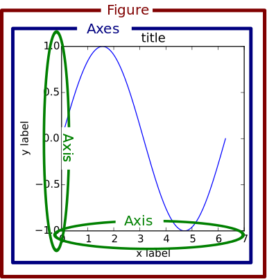
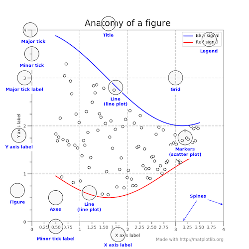
Let's start with an advanced example and then move back to the basics.
import matplotlib.pyplot as plt
import numpy as np

rng = np.arange(50)
rnd = np.random.randint(0, 10, size=(3, rng.size))
yrs = 1950 + rng

fig, ax = plt.subplots(figsize=(5, 3))
ax.stackplot(yrs, rng + rnd, labels=['Eastasia', 'Eurasia', 'Oceania'])
ax.set_title('Combined debt growth over time')
ax.legend(loc='upper left')
ax.set_ylabel('Total debt')
ax.set_xlim(left=yrs[0], right=yrs[-1])
fig.tight_layout()
plt.show()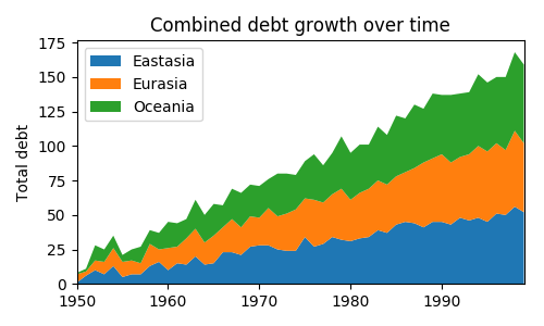
A basic example:
import matplotlib.pyplot as plt
plt.plot([1,2,3,4])
plt.ylabel('some numbers')
plt.show()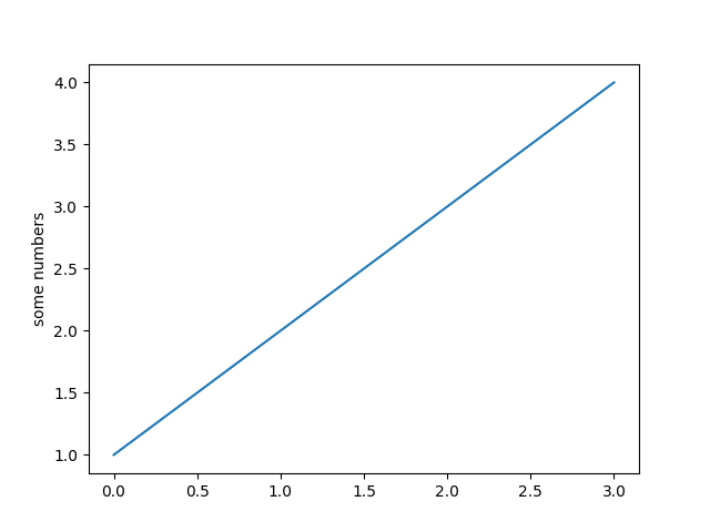
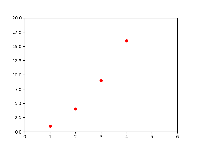
Changing default format ('b-') to red circles ('ro'):
import matplotlib.pyplot as plt
plt.plot([1,2,3,4], [1,4,9,16], 'ro')
plt.axis([0, 6, 0, 20])
plt.show()
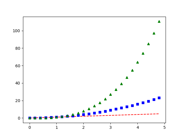
We can have multiple plots in the same axes.
import numpy as np
import matplotlib.pyplot as plt

t = np.arange(0., 5., 0.2)

# red dashes, blue squares and green triangles
plt.plot(t, t, 'r--', t, t**2, 'bs', t, t**3, 'g^')
plt.show()
- Plot the following dataset in Python. Use a blue dashed line. Don't forget to add a title and axis labels!
| Time (decade): | 0 | 1 | 2 | 3 | 4 | 5 | 6 |
| CO2 concentration (ppm): | 250 | 265 | 272 | 260 | 300 | 320 | 389 |
- Repeat the multiple plots in the same figure as a few slides ago, but using the following properties:
- y = t: teal, dotted line
- y = t^2: Yellow, dashed line
- y = t^3: Magenta circles
A few sites that might be useful:
Sample solution 1
import matplotlib.pyplot as plt
times = range(7)
co2 = [250, 265, 272, 260, 300, 320, 389]
#plt.plot(times, co2)
plt.plot(times, co2, 'b--')
plt.title("Concentration of CO2 versus time")
plt.ylabel("[CO2]")
plt.xlabel("Time (decade)")
plt.show()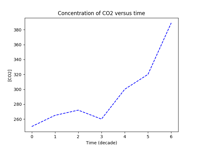
Sample solution 2
import numpy as np
import matplotlib.pyplot as plt

t = np.arange(0., 5., 0.2)

plt.plot(t, t, color='teal', linestyle=':')
plt.plot(t, t**2, 'y--', t, t**3, 'mo')
plt.show()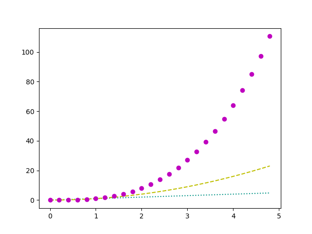
Pandas is a data analysis/manipulation library. It operates on top of the numerical library numpy, so we will start by having a look at it.
>>> import numpy as np
>>> np.zeros(10)
array([0., 0., 0., 0., 0., 0., 0., 0., 0., 0.])
>>> np.full((3,5),1.23)
array([[1.23, 1.23, 1.23, 1.23, 1.23],
       [1.23, 1.23, 1.23, 1.23, 1.23],
       [1.23, 1.23, 1.23, 1.23, 1.23]])
>>> np.arange(0, 20, 2)
array([ 0,  2,  4,  6,  8, 10, 12, 14, 16, 18])
>>> np.linspace(0, 1, 5)
array([0.  , 0.25, 0.5 , 0.75, 1.  ])
>>> np.random.randint(10, size=6)
array([0, 4, 1, 3, 9, 1])
>>> np.random.randint(10, size=(3,4))
array([[0, 3, 5, 7],
       [3, 4, 7, 2],
       [5, 2, 1, 0]])
>>> np.random.randint(10, size=(3,4,5))
array([[[5, 3, 2, 5, 6],
        [2, 6, 0, 2, 3],
        [3, 7, 7, 7, 5],
        [5, 1, 1, 5, 9]],

       [[5, 4, 0, 0, 1],
        [6, 4, 2, 6, 5],
        [6, 1, 7, 4, 8],
        [2, 1, 7, 9, 4]],

       [[7, 1, 9, 2, 7],
        [5, 8, 3, 3, 0],
        [6, 5, 9, 1, 4],
        [0, 4, 7, 8, 4]]])
Indexing and slicing work in the same way as they do for lists.
>>> x1 = np.array([4, 3, 4, 4, 8, 4])
>>> x1[0]
4
>>> x1[-2]
8
>>> x2 = np.array([[3, 7, 5, 5],
...       [0, 1, 5, 9],
...       [3, 0, 5, 0]])
>>> x2[2,3]
0
>>> x2[2,-1]
0
>>> x = np.arange(10)
>>> x[:5]
array([0, 1, 2, 3, 4])
>>> x[4:7]
array([4, 5, 6])
Numpy arrays can be concatenated and split in many different ways.
>>> x = np.array([1, 2, 3])
>>> y = np.array([3, 2, 1])
>>> z = [21,21,21]
>>> np.concatenate([x, y,z])
array([ 1,  2,  3,  3,  2,  1, 21, 21, 21])
>>> x = np.array([3,4,5])
>>> grid = np.array([[1,2,3],[17,18,19]])
>>> np.vstack([x,grid])
array([[ 3,  4,  5],
       [ 1,  2,  3],
       [17, 18, 19]])
>>> z = np.array([[9],[9]])
>>> np.hstack([grid,z])
array([[ 1,  2,  3,  9],
       [17, 18, 19,  9]])
>>> grid = np.arange(16).reshape((4,4))
>>> grid
array([[ 0,  1,  2,  3],
       [ 4,  5,  6,  7],
       [ 8,  9, 10, 11],
       [12, 13, 14, 15]])
>>> upper,lower = np.vsplit(grid,[2])
>>> print (upper, lower)
(array([[0, 1, 2, 3],
       [4, 5, 6, 7]]), array([[ 8,  9, 10, 11],
       [12, 13, 14, 15]]))
The main Pandas structure we will be interested in is the DataFrame.
import pandas as pd
data = pd.DataFrame({'Country': ['Russia','Colombia','Chile','Equador','Nigeria'],
                    'Rank':[121,40,100,130,11]})
print(data)

    Country  Rank
0    Russia   121
1  Colombia    40
2     Chile   100
3   Equador   130
4   Nigeria    11
A quick way of having a summary of the statistics your data set is using the describe() method.
data.describe()
             Rank
count    5.000000
mean    80.400000
std     52.300096
min     11.000000
25%     40.000000
50%    100.000000
75%    121.000000
max    130.000000
Of course, that will only give you information about the numeric fields of your dataset. If you want more general information, use info().
>>> data.info()

RangeIndex: 5 entries, 0 to 4
Data columns (total 2 columns):
Country    5 non-null object
Rank       5 non-null int64
dtypes: int64(1), object(1)
memory usage: 160.0+ bytes
We can, of course, sort the data set.
>>> data.sort_values(by=['Rank'],ascending=True,inplace=False)
    Country  Rank
4   Nigeria    11
1  Colombia    40
2     Chile   100
0    Russia   121
3   Equador   130
You can sort by more than one column.
>>> data = pd.DataFrame({'k1':['one']*3 + ['two']*4 + ['one']*2, 'k2':[2,1,3,3,3,4,4,2,5]})
>>> data
    k1  k2
0  one   2
1  one   1
2  one   3
3  two   3
4  two   3
5  two   4
6  two   4
7  one   2
8  one   5
>>> data.sort_values(by=['k1','k2'],ascending=[True,False],inplace=False)
    k1  k2
8  one   5
2  one   3
0  one   2
7  one   2
1  one   1
5  two   4
6  two   4
3  two   3
4  two   3
Removing duplicates is very easy!
>>> data.drop_duplicates()
    k1  k2
0  one   2
1  one   1
2  one   3
3  two   3
5  two   4
8  one   5
This is how you create a new variable based on a combination of the existing ones:
>>> data.assign(new_variable = data['k2']*20)
    k1  k2  new_variable
0  one   2            40
1  one   1            20
2  one   3            60
3  two   3            60
4  two   3            60
5  two   4            80
6  two   4            80
7  one   2            40
8  one   5           100
Now, let's try binning some data.
data = pd.DataFrame({'names':['Alice','Bob','Charlie','Dan','Eve','Frank','Grace','Heidi','Judy','Michael','Oscar','Pat'], 'ages':[20, 22, 25, 27, 21, 23, 37, 31, 61, 45, 41, 32]})
>>> data
      names  ages
0     Alice    20
1       Bob    22
2   Charlie    25
3       Dan    27
4       Eve    21
5     Frank    23
6     Grace    37
7     Heidi    31
8      Judy    61
9   Michael    45
10    Oscar    41
11      Pat    32
>>> bins = [18, 25, 35, 60, 100]
>>> brackets = pd.cut(data['ages'],bins)
>>> brackets
0      (18, 25]
1      (18, 25]
2      (18, 25]
3      (25, 35]
4      (18, 25]
5      (18, 25]
6      (35, 60]
7      (25, 35]
8     (60, 100]
9      (35, 60]
10     (35, 60]
11     (25, 35]
Name: ages, dtype: category
Categories (4, interval[int64]): [(18, 25] < (25, 35] < (35, 60] < (60, 100]]
>>> pd.value_counts(brackets)
(18, 25]     5
(35, 60]     3
(25, 35]     3
(60, 100]    1
Name: ages, dtype: int64
A very useful operation for datasets is grouping data and creating summaries.
>>> df = pd.DataFrame({'key1' : ['a', 'a', 'b', 'b', 'a'],
                   'key2' : ['one', 'two', 'one', 'two', 'one'],
                   'data1' : np.random.randn(5),
                   'data2' : np.random.randn(5)})
>>> df
  key1 key2     data1     data2
0    a  one -0.369708 -1.215059
1    a  two -0.341208 -0.884716
2    b  one -0.672269  0.149367
3    b  two -1.468556  1.386700
4    a  one -0.366804 -0.634380
>>> grouped = df['data1'].groupby(df['key1'])

>>> grouped.mean()
key1
a   -0.359240
b   -1.070413
Name: data1, dtype: float64
There are many, many ways of accessing specific subsets of our data set.
>>> dates = pd.date_range('20130101',periods=6)
>>> df = pd.DataFrame(np.random.randn(6,4),index=dates,columns=list('ABCD'))
>>> df
                   A         B         C         D
2013-01-01  0.482837  0.005617  1.011802 -0.817221
2013-01-02 -1.351376  0.552897  0.503408 -0.431504
2013-01-03 -0.244983 -0.470076 -0.489829 -0.763309
2013-01-04  0.019689 -1.759921  0.740204  0.763700
2013-01-05  0.607637  1.679538 -0.599785 -0.365752
2013-01-06  1.371928 -1.148383 -1.586073  0.784124

>>> df[:3]
                   A         B         C         D
2013-01-01  0.482837  0.005617  1.011802 -0.817221
2013-01-02 -1.351376  0.552897  0.503408 -0.431504
2013-01-03 -0.244983 -0.470076 -0.489829 -0.763309
>>> df['20130101':'20130104']
                   A         B         C         D
2013-01-01  0.482837  0.005617  1.011802 -0.817221
2013-01-02 -1.351376  0.552897  0.503408 -0.431504
2013-01-03 -0.244983 -0.470076 -0.489829 -0.763309
2013-01-04  0.019689 -1.759921  0.740204  0.763700
There are many, many ways of accessing specific subsets of our data set.
>>> df.loc[:,['A','B']]
                   A         B
2013-01-01  0.482837  0.005617
2013-01-02 -1.351376  0.552897
2013-01-03 -0.244983 -0.470076
2013-01-04  0.019689 -1.759921
2013-01-05  0.607637  1.679538
2013-01-06  1.371928 -1.148383
>>> df.loc['20130102':'20130103',['A','B']]
                   A         B
2013-01-02 -1.351376  0.552897
2013-01-03 -0.244983 -0.470076
>>> df[df.A > 1]
                   A         B         C         D
2013-01-06  1.371928 -1.148383 -1.586073  0.784124
>>> df.query('A > C')
                   A         B         C         D
2013-01-03 -0.244983 -0.470076 -0.489829 -0.763309
2013-01-05  0.607637  1.679538 -0.599785 -0.365752
2013-01-06  1.371928 -1.148383 -1.586073  0.784124
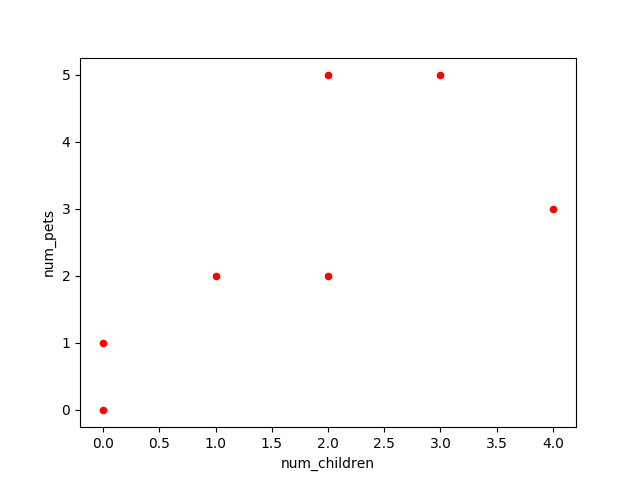
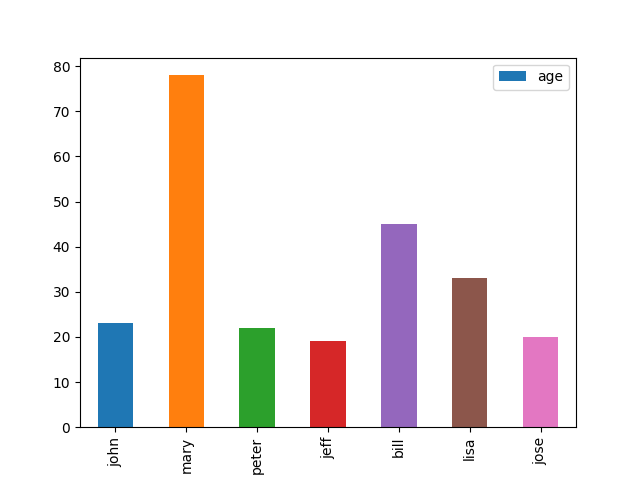
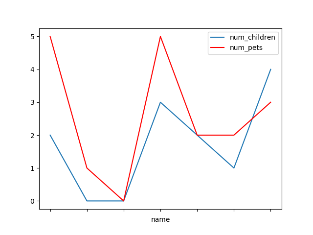
Pandas can do plotting, too!
>>> df = pd.DataFrame({
    'name':['john','mary','peter','jeff','bill','lisa','jose'],
    'age':[23,78,22,19,45,33,20],
    'gender':['M','F','M','M','M','F','M'],
    'state':['california','dc','california','dc','california','texas','texas'],
    'num_children':[2,0,0,3,2,1,4],
    'num_pets':[5,1,0,5,2,2,3]
})
>>> import matplotlib.pyplot as plt
>>> df.plot(kind='scatter',x='num_children',y='num_pets',color='red')
<matplotlib.axes._subplots.AxesSubplot object at 0x7f56722e22e8>
>>> plt.show()
>>> df.plot(kind='bar',x='name',y='age')
<matplotlib.axes._subplots.AxesSubplot object at 0x7f56722e22e8>
>>> plt.show()
>>> fig, ax = plt.subplots()
>>> df.plot(kind='line',x='name',y='num_children',ax=ax)
<matplotlib.axes._subplots.AxesSubplot object at 0x7f56622145c0>
>>> df.plot(kind='line',x='name',y='num_pets', color='red', ax=ax)
<matplotlib.axes._subplots.AxesSubplot object at 0x7f56622145c0>
>>> plt.show()
CSV files are pandas' best friend. Try this with cereal.csv:
>>> import os
>>> os.chdir('Whatever directory you\'ve saved cereal.csv in')

>>> df = pd.read_csv('cereal.csv')
>>> df.head(5)
                        name mfr type    ...      weight  cups     rating
0                  100% Bran   N    C    ...         1.0  0.33  68.402973
1          100% Natural Bran   Q    C    ...         1.0  1.00  33.983679
2                   All-Bran   K    C    ...         1.0  0.33  59.425505
3  All-Bran with Extra Fiber   K    C    ...         1.0  0.50  93.704912
4             Almond Delight   R    C    ...         1.0  0.75  34.384843

[5 rows x 16 columns]
You can also easily save a dataframe as a CSV file:
>>> df.to_csv('cereal_copy.csv')
Do you see any difference between the copies?
- Write a Python program to plot all the data in fdata.csv.
- Write a Python program to create a 5x5 numpy array with 1 on the border and 0 inside.
- Write a Python program to create a 5x5 array with random values and find the minimum and maximum values.
- Write a Python program to iterate over rows in a DataFrame.
A few sites that might be useful:
Sample solution 1
import matplotlib.pyplot as plt
import pandas as pd
import os
os.chdir('Whatever directory you\'ve saved fdata.csv in')
df = pd.read_csv('fdata.csv')
df.plot(x="Date",y=["Open", "High", "Low", "Close"])
plt.show()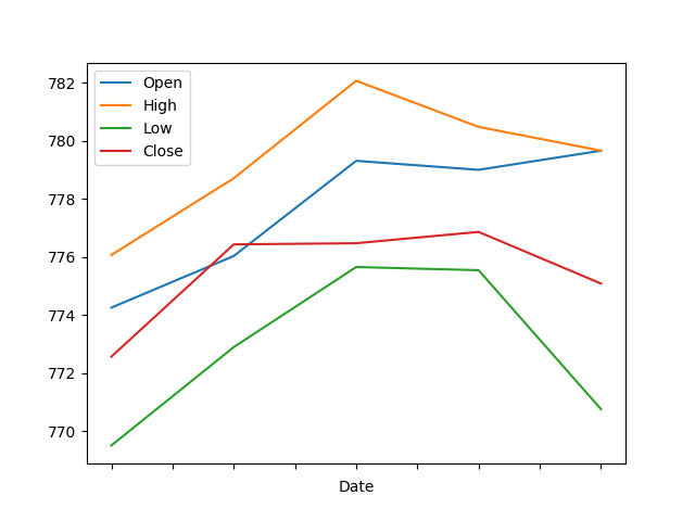
Sample solution 2
import numpy as np
x = np.ones((5,5))
x[1:-1,1:-1] = 0
print(x)

[[1. 1. 1. 1. 1.]
 [1. 0. 0. 0. 1.]
 [1. 0. 0. 0. 1.]
 [1. 0. 0. 0. 1.]
 [1. 1. 1. 1. 1.]]
Sample solution 3
import numpy as np
x = np.random.random((5,5))
print("Original Array:")
print(x)
xmin, xmax = x.min(), x.max()
print("Minimum and Maximum Values:")
print(xmin, xmax)

Original Array:
[[0.96108746 0.66272609 0.42670443 0.5463886  0.13583066]
 [0.78215537 0.29811248 0.26380749 0.93835562 0.00176633]
 [0.09763454 0.52875892 0.71247172 0.7065642  0.76375718]
 [0.7768379  0.85771292 0.17135697 0.83372476 0.83760277]
 [0.20412887 0.9024384  0.68057959 0.38648805 0.62763643]]
Minimum and Maximum Values:
0.0017663346508800526 0.9610874575010275
Sample solution 4
import pandas as pd
import os
os.chdir('Whatever directory you\'ve saved cereal.csv in')

df = pd.read_csv('cereal.csv')
for index, row in df.iterrows():
    print(row['name'], row['calories'])

100% Bran 70
100% Natural Bran 120
All-Bran 70
All-Bran with Extra Fiber 50
Almond Delight 110
Apple Cinnamon Cheerios 110
Apple Jacks 110
(...)
Thank you for your attention!
We will send you a survey for feedback; please take 2 minutes to answer, it helps us a lot!