Introduction to Image Analysis with Fiji
Erick Martins Ratamero
Research Fellow
- These slides: http://tiny.cc/camduIA (redirects to https://erickmartins.github.io/ImageAnalysis.html)
- Navigation: arrow keys left and right to navigate
- 'm' key to get to navigation menu
- Escape for slide overview
- Where to find help after the workshop (links also available on the menu):
- HUGE thanks to Dave Mason (formerly) from the University of Liverpool
- You can find his original slides at https://pcwww.liv.ac.uk/~dnmason/ia.html (and then realise they look very much like these)
Throughtout the presentation, test data will look like this: 01-Photo.tif
Commands on the Fiji menu will look like: [File > Save]
How an Image is formed
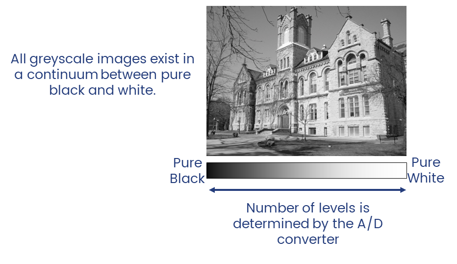
Understanding digital images
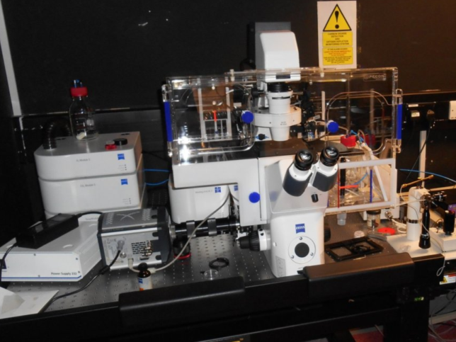
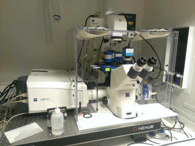
Widefield and Confocal microscopes acquire images in different ways.
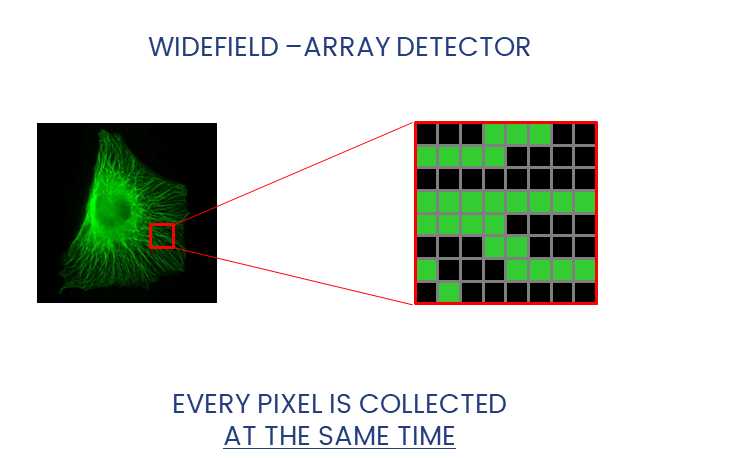
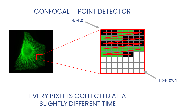
Widefield and laser-scanning microscopes acquire images in different ways.
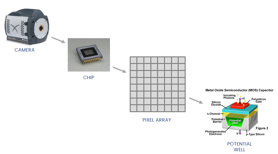
Detectors collect photons and convert them to a voltage
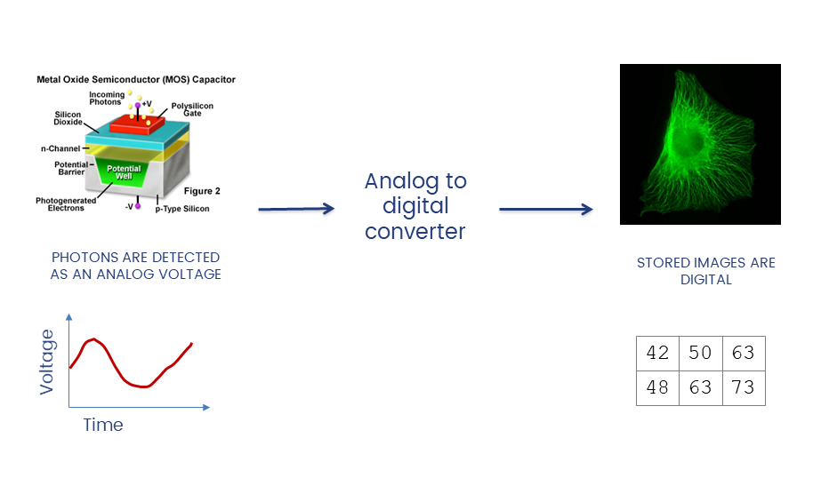
The A/D converter determines the dynamic range of the data
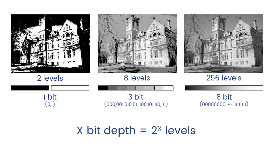
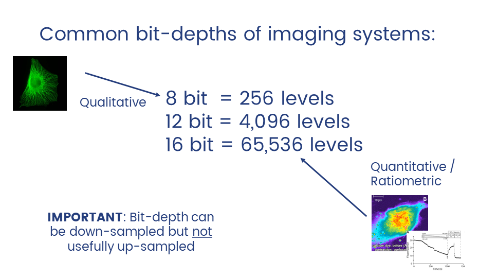
Unless you have good reason not to, always collect data at the highest possible bit depth
32 bit is a special data type called floating point.
TL;DR: pixels can have non-integer values which can be useful in applications like ratiometric imaging.
Introduction to ImageJ & Fiji
A cross platform, open source, Java-based image processing program

- Open Source (free to modify)
- Extensible (plugins)
- Cross-Platform (Java-Based)
- Scriptable for Automation
- Vast Functionality
- Includes the Bioformats Library
ImageJ is a java program for image processing and analysis.
Fiji extends this via plugins.
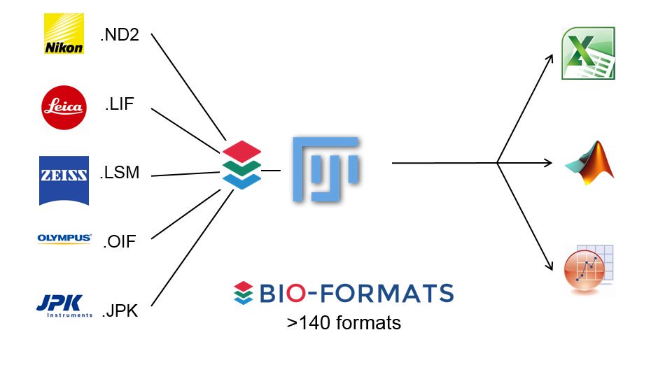
Learn more about Bio-Formats here
Hands on With Fiji
Getting to know the interface, info & status bars, calibrated vs non-calibrated images
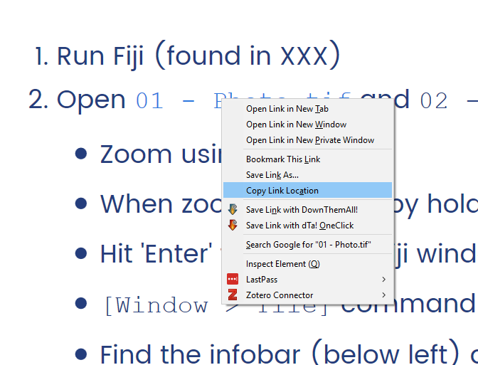
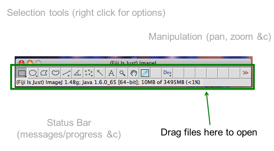
- Run Fiji (Look for the shortcut on your desktop)
- Open
01-Photo.tifand02-Biological_Image.tif - Zoom using +/- keys
- When zoomed in, pan by holding space and click-dragging with mouse
- Hit 'Enter' to bring the Fiji window to the front
[Window > Tile]command is very useful when opening multiple images- Find:
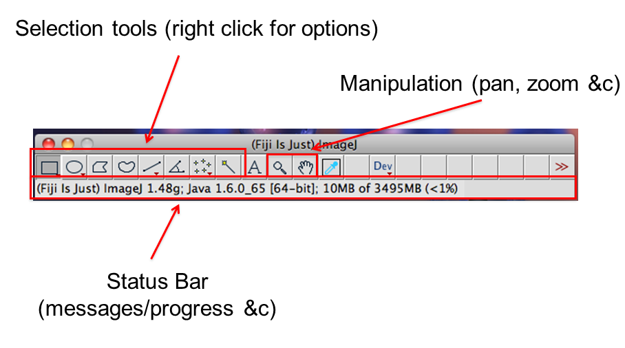
- infobar (left top): gives info on the image
- statusbar (right bottom): gives current cursor coordinates and intensity readout
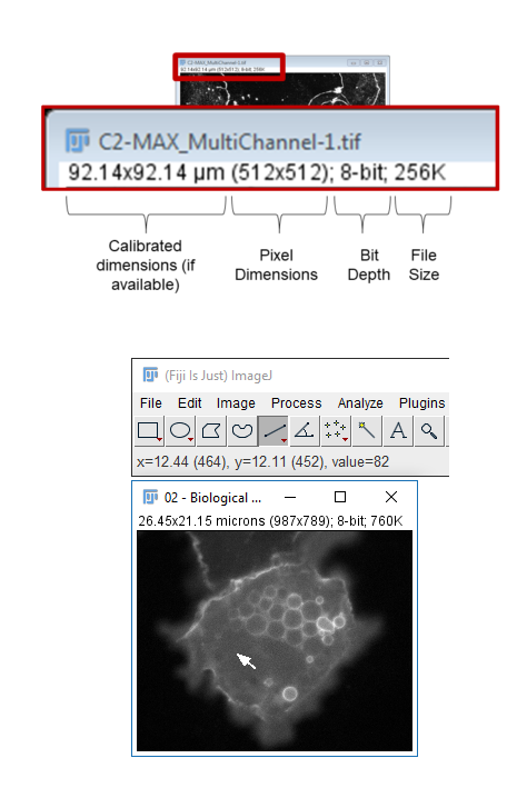
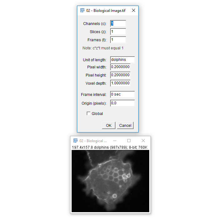
- The Infobar is a great way to tell if your image is calibrated
- Running
[Image > Properties]also allows you to view and set calibration - The spatial calibration can be in any unit you like but (almost) all subsequent measurements will use that unit!
- For μm, use
umormicron
Basic Manipulations
Intensity and Geometric adjustments
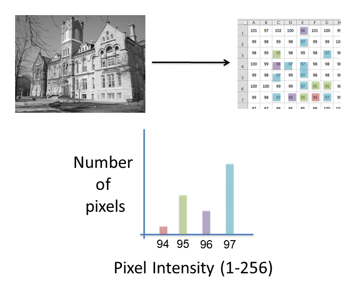
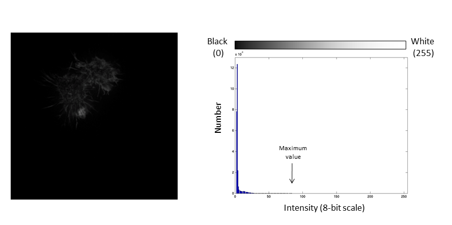
Images are an array of intensity values. The intensity histogram shows the number (on the y-axis) of each intensity value (on the x-axis) and thus the distribution of intensities
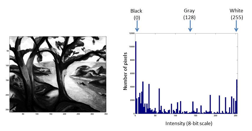
Photos typically have a broad range of intensity values and so the distribution of intensities varies greatly
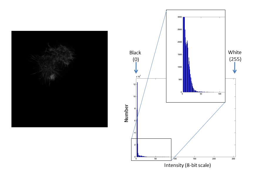
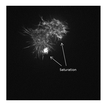
Fluorescent micrographs will typically have a much more predicatble distribution:
The Black and White points of the histogram dictate the bounds of the display (changing these values alters the brightness and contrast of the image)
- Brightness: horizontal position of the display window
- Contrast: distance between the black and white point
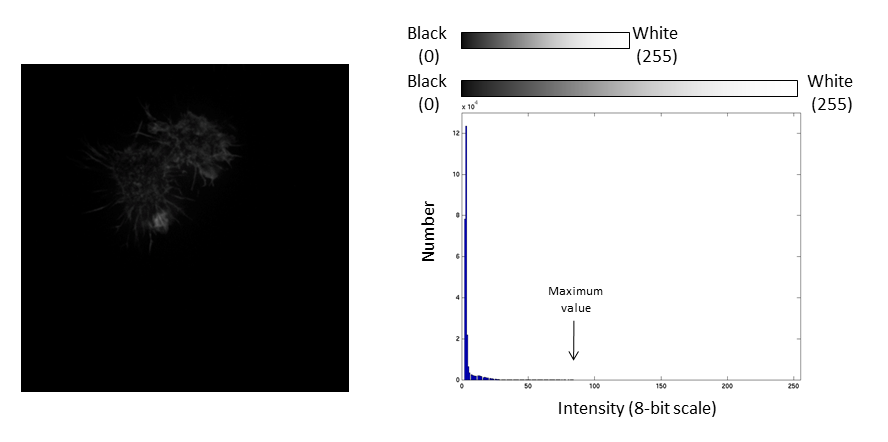
The histogram is now stretched and the intensity value of every pixel is effectively doubled which increases the contrast in the image
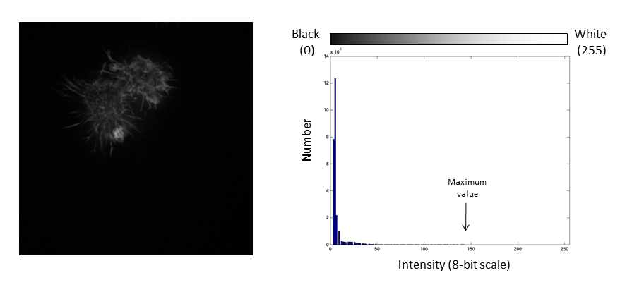
If we repeat the same manipulation, the maximum intensity value in the image is now outside the bounds of the display scale!
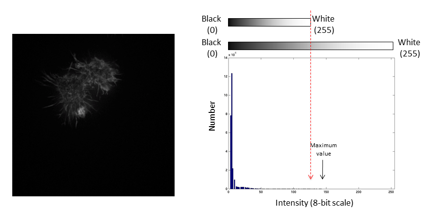
Values falling beyond the new White point are dumped into the top bin of the histogram (IE 256 in an 8-bit image) and information from the image is lost
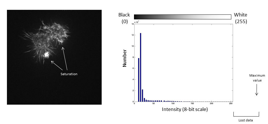
Be warned: removing information from an image is deemed an unacceptable maniplulation and can constitute academic fraud!
For an excellent (if slightly dated) review of permissible image manipulation see:Rossner & Yamada (2004): "What's in a picture? The temptation of image manipulation"
The best advice is to get it right during acquisition!
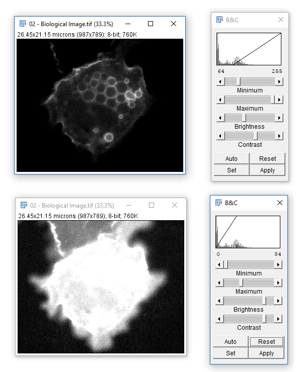
- Open
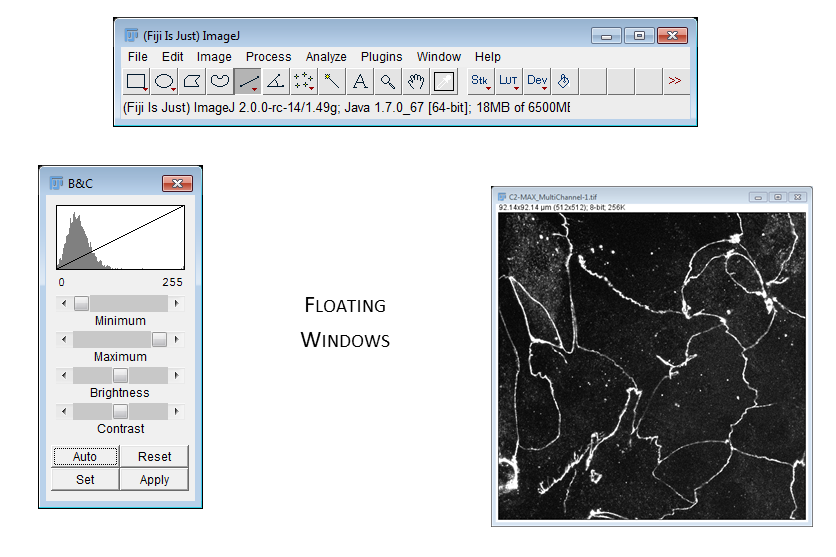
02-Biological Image.tif - Run
[Image > Adjust > Brightness & Contrast] - The top two bars adjust the Black and White points
- All data below the black point or above the white point become black or white respectively! (and are thus underexposed or saturated)
- Reset will stretch to the range of the bit depth (ish)
- Set lets you define black and white points
- Apply writes in adjustments (never ever ever use on the original image, and even on a copy proceed with care!)
- You can also use
[Process > Enhance Contrast]to autocontrast
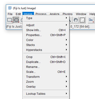
[Image > Crop]: Reduce the canvas size to current area selection[Image > Duplicate]: Duplicate the selected window/stack or selection[Image > Rename]: Change the title of the window[Image > Scale]: Scale the image pixels up or down (calibration is also scaled)
Measurements
Making measurements, what to measure, line vs area
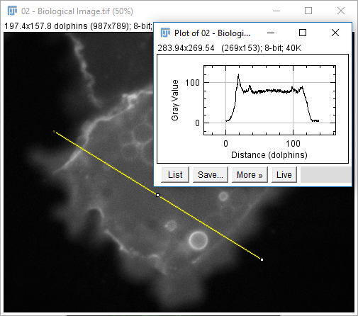
- Open
02-Biological Image.tif - Select Line Selection tool (fifth tool from left)
- Draw a line (shift sets 45° increments)
- Hit 'm' or run
[Analyze > Measure] - Run
[Analyze > Plot Profile]
The measurements provided are set via [Analyze > Set Measurements...] except for selection-specific measurements (length, angle, coords)
- Open
02-Biological Image.tif - Select rectangle Selection tool (first tool from left)
- Draw a rectangle (shift / ctrl modify)
- Hit 'm' or run
[Analyze > Measure]
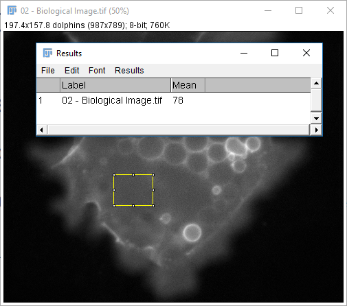
The measurements provided are set via [Analyze > Set Measurements...] except for selection-specific measurements (length, angle, coords)
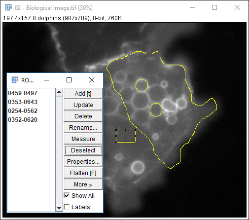
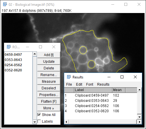
The ROI manager is used to store and measure selections
- Open
02-Biological Image.tif - Make a selection (any type)
- Hit 't' or run
[Edit > Selection > Add to Manager] - Repeat several times
- Run
[More > Multi-measure] - Use
[More > Save]for better data provenance!
Scale Bars and Colour modes
Adding a scale bar, changing the colour mode
- Open
02-Biological Image.tif - Check the image is calibrated (infobar or
[Image > Properties]) - Run
[Analyze > Tools > Scale Bar] - Pick a non-white colour for the scale bar
- Hit OK
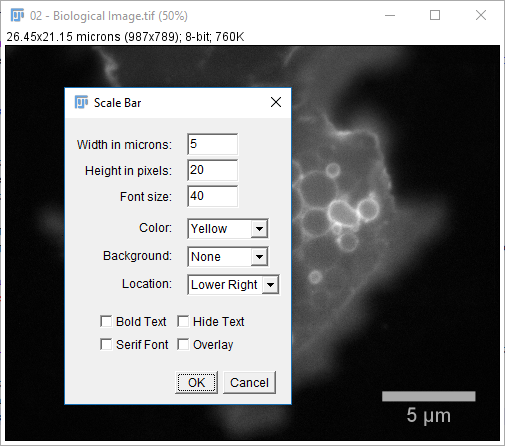
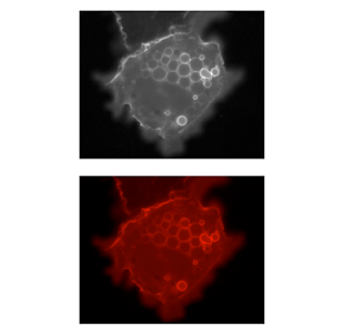
What Happened to our yellow scale bar?
Open the Original image
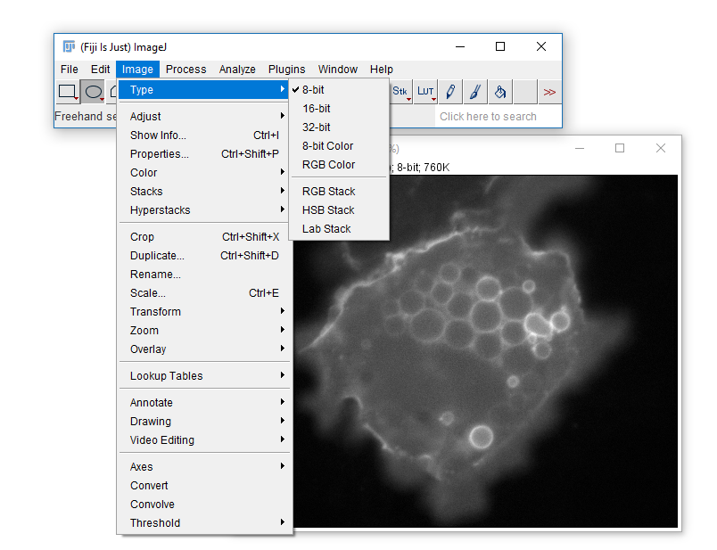
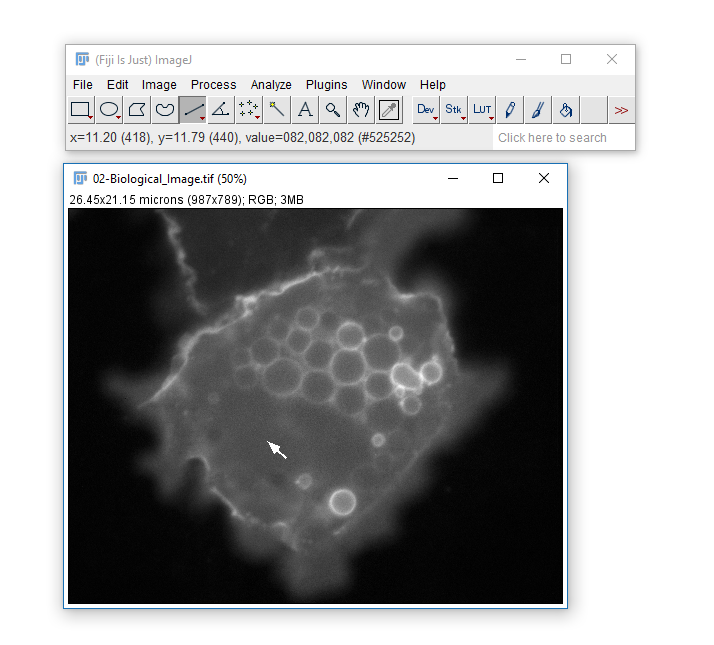
Run [Image > Type > RGB Color]
Try adding a scale bar again
More on scale bars here. For another way to approach this, see Overlays
Stacks
Understanding how Fiji deals with multidimensional images
Some file formats (eg. TIF) can store multiple images in one file which are called stacks
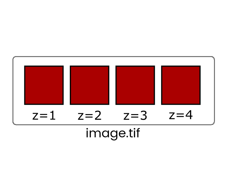
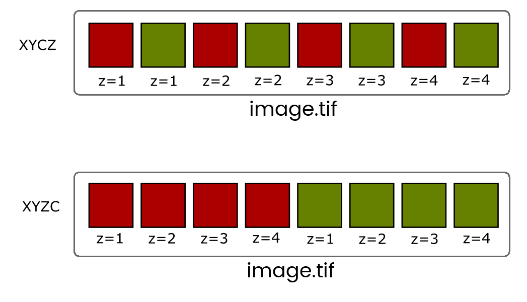
When more than one dimension (time, z, channel) is included, the images are still stored in a linear stack so it's critical to know the dimension order (eg, XYCZT, XYZTC etc) so you can navigate the stack correctly.
You will very rarely have to deal with Interleaved stacks because of Hyperstacks which give you independent control of dimensions with additional control bars.
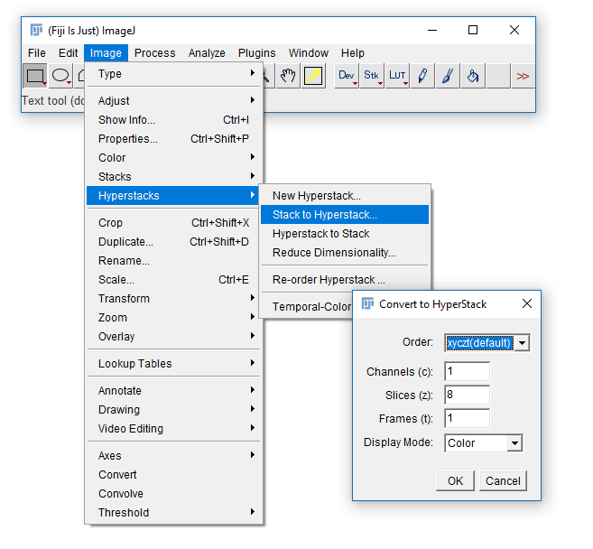
Convert between stack types with the [Image > Hyperstack] menu
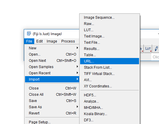
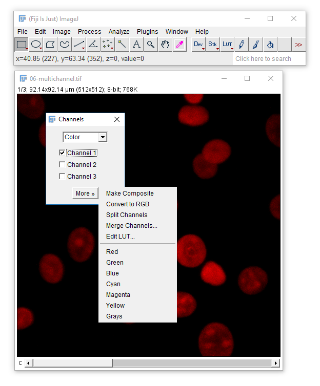
- Open
06-MultiChannel.tif - (If opening via URL run
[Image > Hyperstacks > Stack to Hyperstack]) - Navigate through the channels then run Channels Tool
[Image > Color > Channels Tool]and change to Greyscale
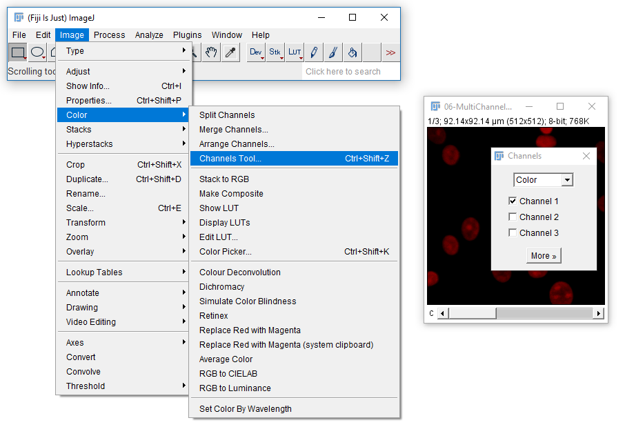
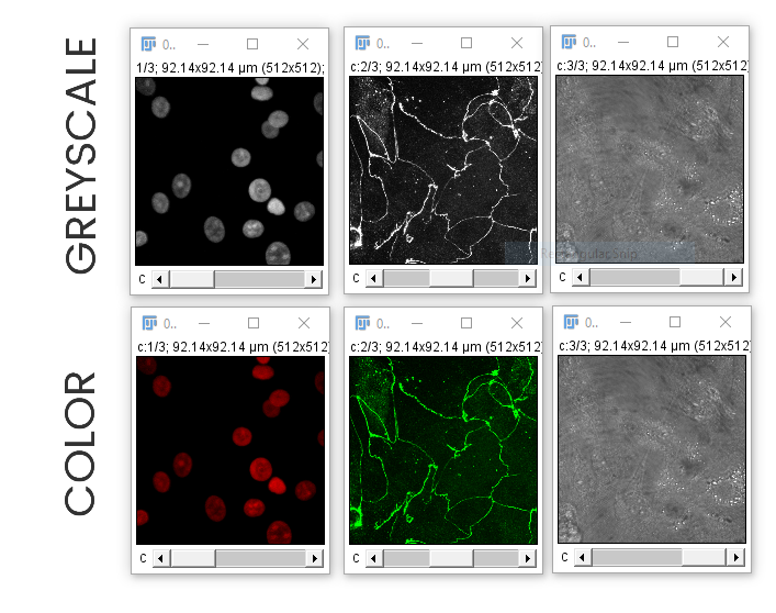
In this image, each channel already has an associated Look Up Table (LUT)
Change to Composite mode
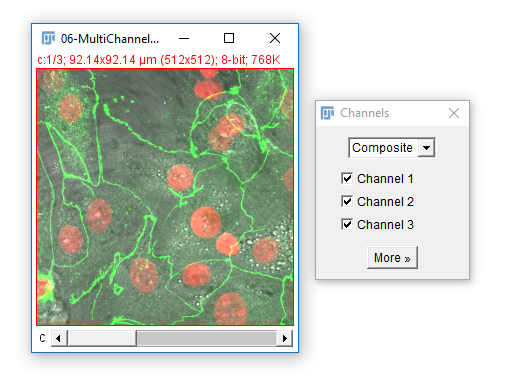
- Use the check boxes (channels tool) to turn channels off
- Navigate through the channels. What happens?
- Adjust the Black and White Points
[Image > Adjust > Brightness & Contrast] - Draw a ROI on a bright area and Measure ('m')
IMPORTANT! The nav bar still selects the active channel, and that is where measurements / maniplulations are applied!
The infobar text, slider and 1px coloured image border all indicate which channel is selected.
Colour in Digital Imaging
What is colour? How and when to use LUTs
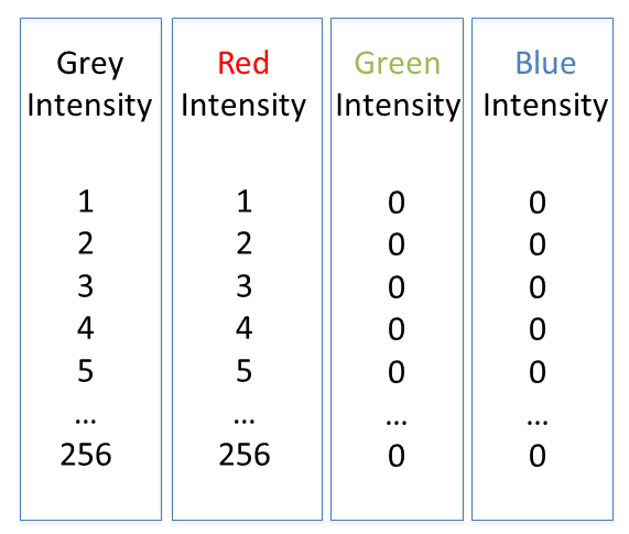
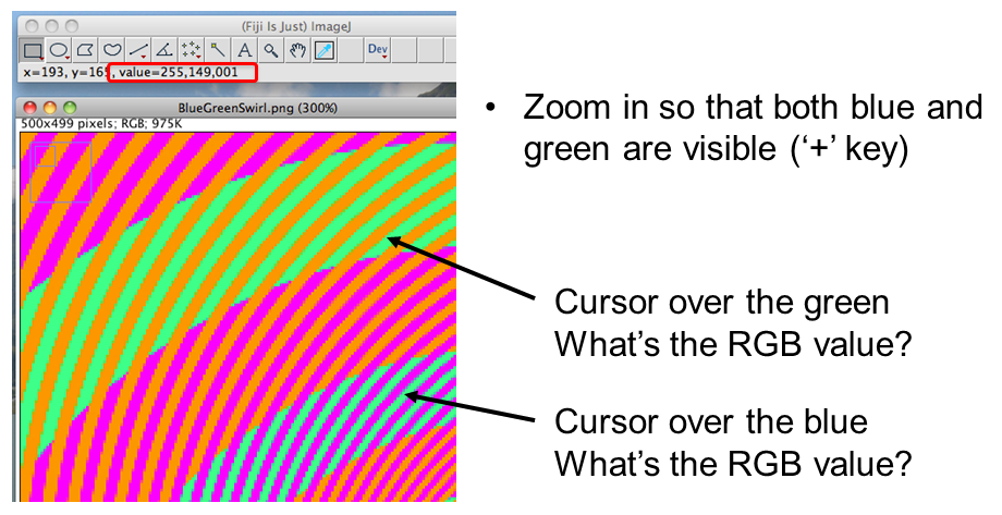
Colour in your images is (almost always) dictated by arbitrary lookup tables
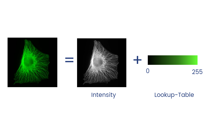
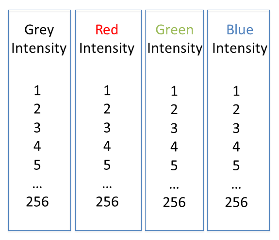
Lookup tables (LUTs) translate an intensity (1-256 for 8 bit) to an RGB display value
Colour in your images is (almost always) dictated by arbitrary lookup tables
Lookup tables (LUTs) translate an intensity (1-256 for 8 bit) to an RGB display value
You can use whatever colours you want (they are arbitrary after all), but the most reliable contrast is greyscale
More info on colour and sensitivity of the human eye here
Additive and Subtractive Colours can be mixed in defined ways
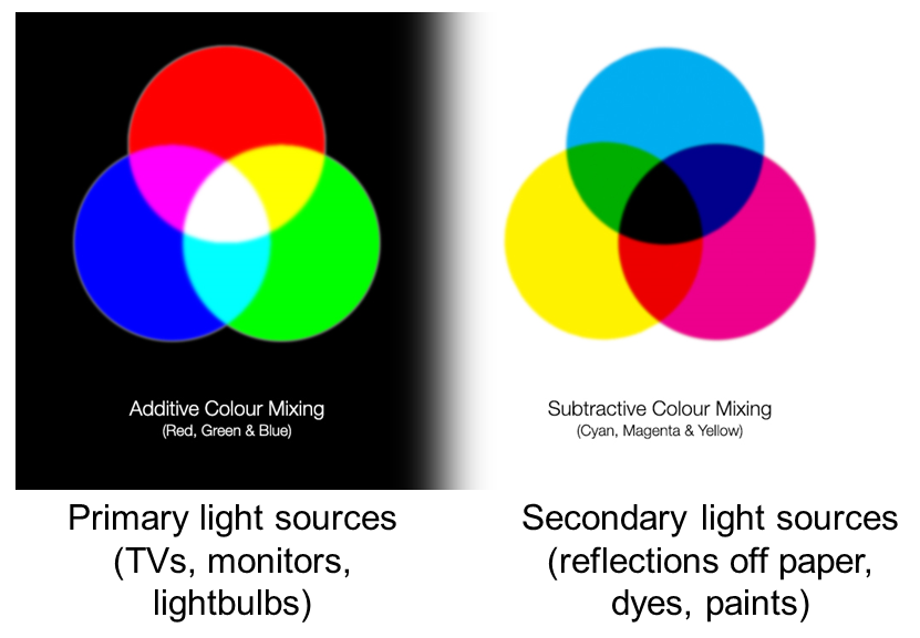
Non 'pure' colours cannot be combined in reliable ways (as they contain a mix of other channels)
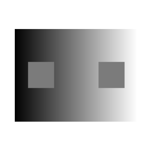
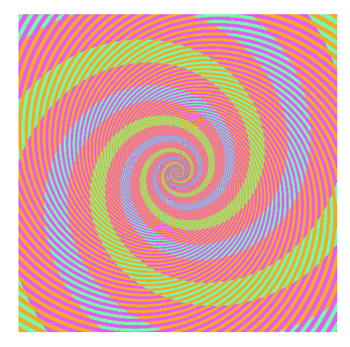
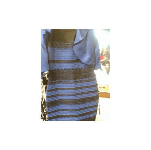
BUT! Interpretation is highly context dependent!
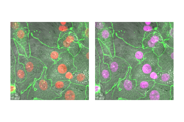
~10% of the population have trouble discerning Red and Green. Consider using Green and Magenta instead which still combine to white.
- Open
06-MultiChannel.tif - (If opening via URL run
[Image > Hyperstacks > Stack to Hyperstack]) - Run
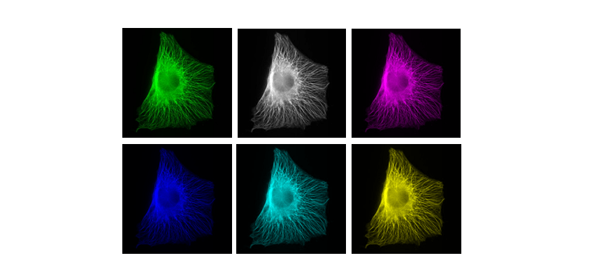
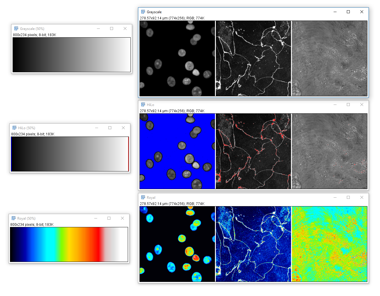
[Image > Lookup Tables], try a few different ones - Run Channels Tool
[Image > Color > Channels Tool], make sure you're in Color or Composite mode, hit More, select a LUT - Run
[Image > Color > Display LUTs]to see all the LUTs on your version of Fiji
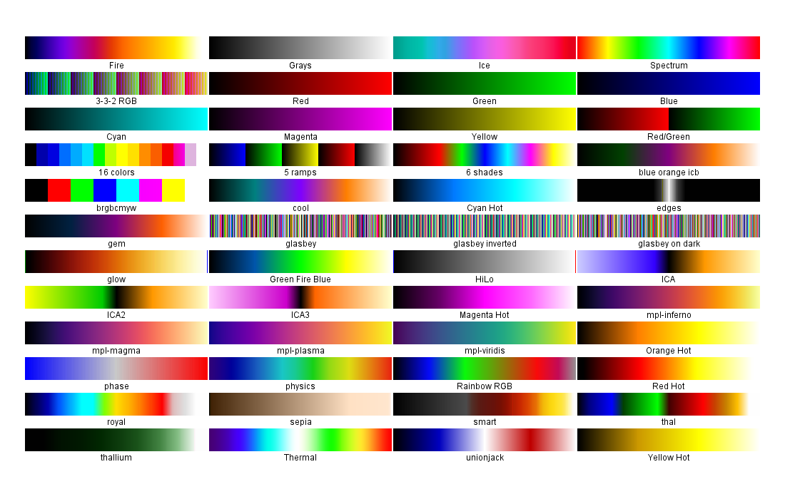
A couple of useful LUTs:
Applications
Applications: Segmentation
What is segmentation? thresholding, Connected Component Analysis
Fiji has an odd way of dealing with masks
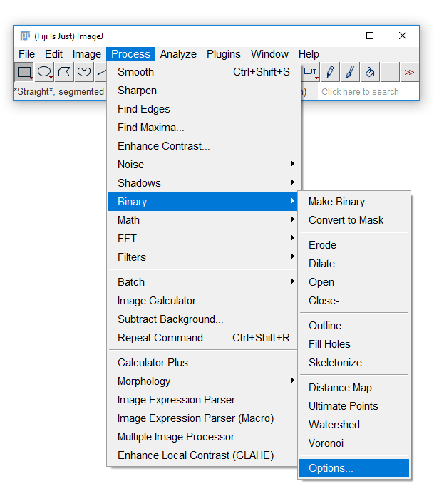
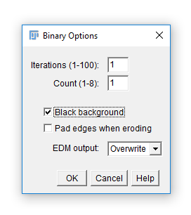
Run [Process > Binary > Options] and check Black Background. Hit OK.
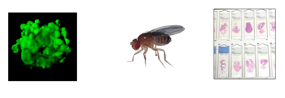
Segmentation is the separation of an image into areas of interest and areas that are not of interest
The end point for most segmentation is a binary mask (false/true, 0/255)
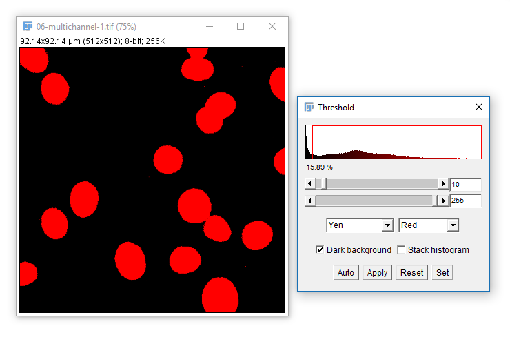
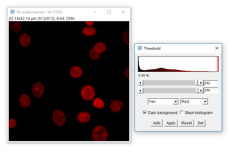
For most applications, intensity-based thresholding works well. This relies on the signal being higher intensity than the background.
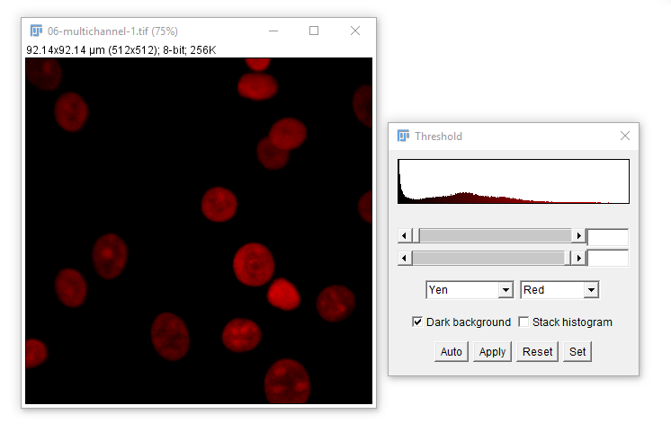
We use a Threshold to pick a cutoff.
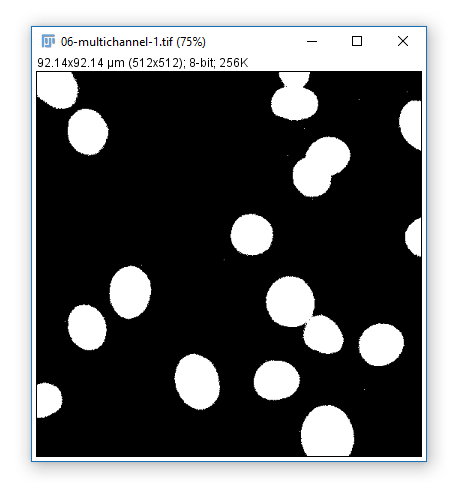
- Open
07-nuclei.tif - Run
[Image > Adjust > Threshold] - Set the lower threshold to 0, 10 and 253, note how the image changes.
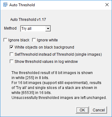
Sometimes you will want to automatically set a threshold. Use the dropdown and Auto button
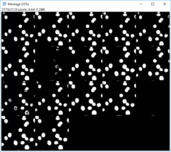
You can trial all autothresholding methods using [Image > Adjust > Auto Threshold] and select 'Try All'
Hit 'Apply' to create a mask based on the current Threshold
What can you do with a mask?
- Count
- Measure
- Visualise
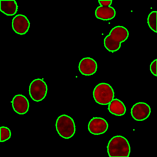
Connected component analysis (CCA) is used to identify contiguous objects in a mask
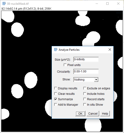
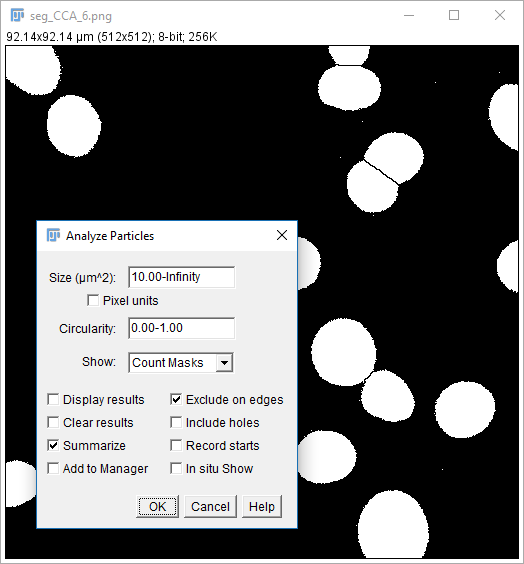
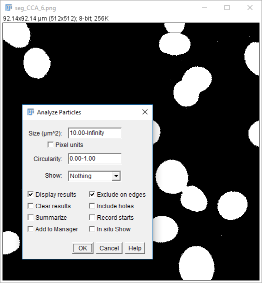
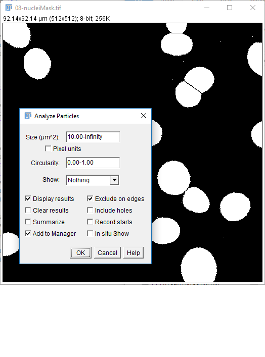
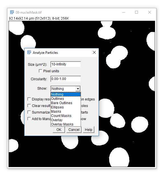
- Open
08-nucleiMask.tif(or use yours from the last step) - Run
[Analyze > Analyze Particles] - Use the settings on the right, hit OK
- You should have a results table with a Count of 31 (you may also have some other stats but we'll come to these later)
But...there are at least 3 problems with this:
- Single pixel spots are counted as objects
- Edge nuclei are counted
- Some nuclei are touching
A quick fix for separating partially-touching roughly circular objects is to use [Process > Binary > Watershed] before running CCA
Analyze Particles comes with the option to Display Results
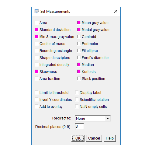
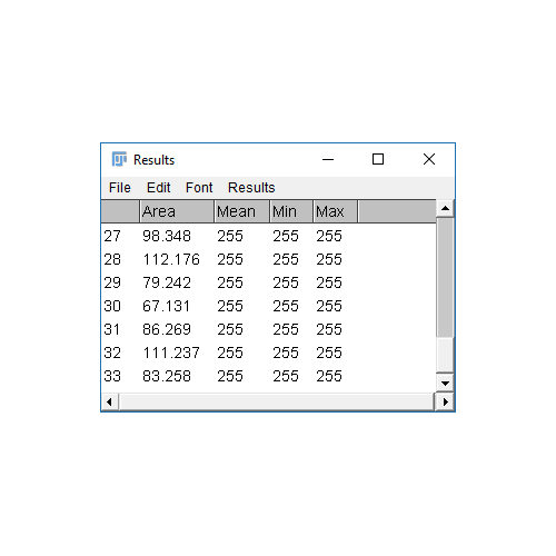
- The results table will have a column for anything selected in
[Analyze > Set Measurements]and one row per object - Measurements (including intensity - labelled purple above) are made on the mask!
To apply measurements to the original image: check Add to Manager in Analyze Particles, open the original image, then run [More > Multi Measure]
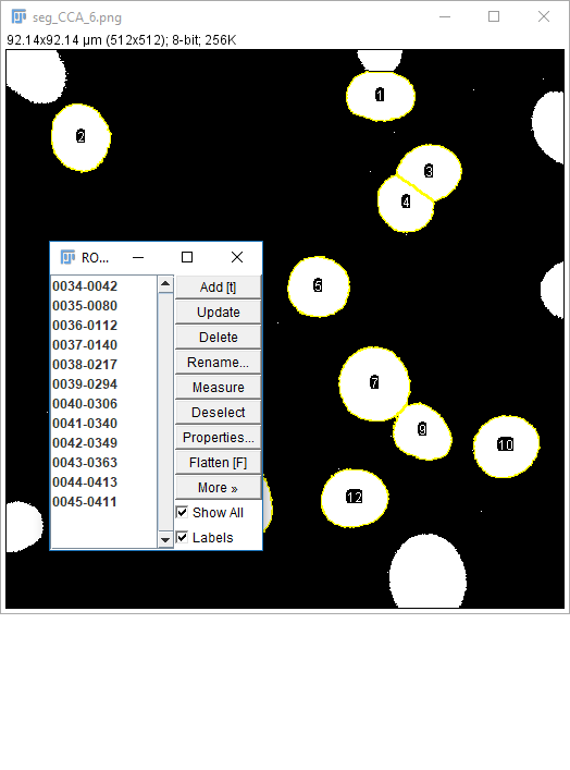
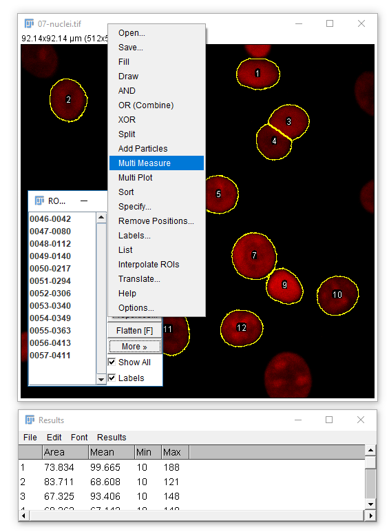
Don't forget [Analyze > Set Measurements] to pick parameters
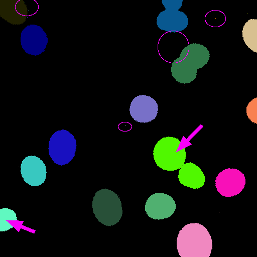
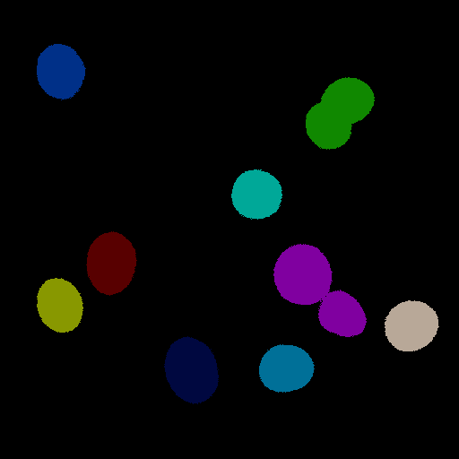
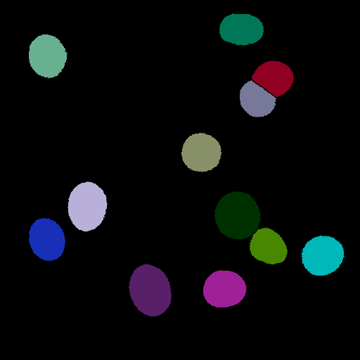
You may want to create an output or display image showing the results of CCA or segmentation. Analyze particles has several useful outputs:
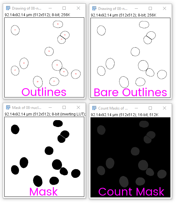
Count masks are very useful in combination with [Image > Look Up Tables > Glasbey]-style (IE random) LUTs
Another trick is to turn the mask into a composite selection then draw it into the original
- Open
08-nucleiMask.tif - Run
[Edit > Selection > Create Selection] - If the black area is selected, run
[Edit > Selection > Make Inverse]. Add it to the ROI manager ('t') - Open the
original image - Convert it to RGB
[Image > Type > RGB Color](remember what happened with the Scale Bar?) - Select the ROI, then run
[Edit > Draw](this will use the current foreground colour and line width)
Example visualisation of woundhealing
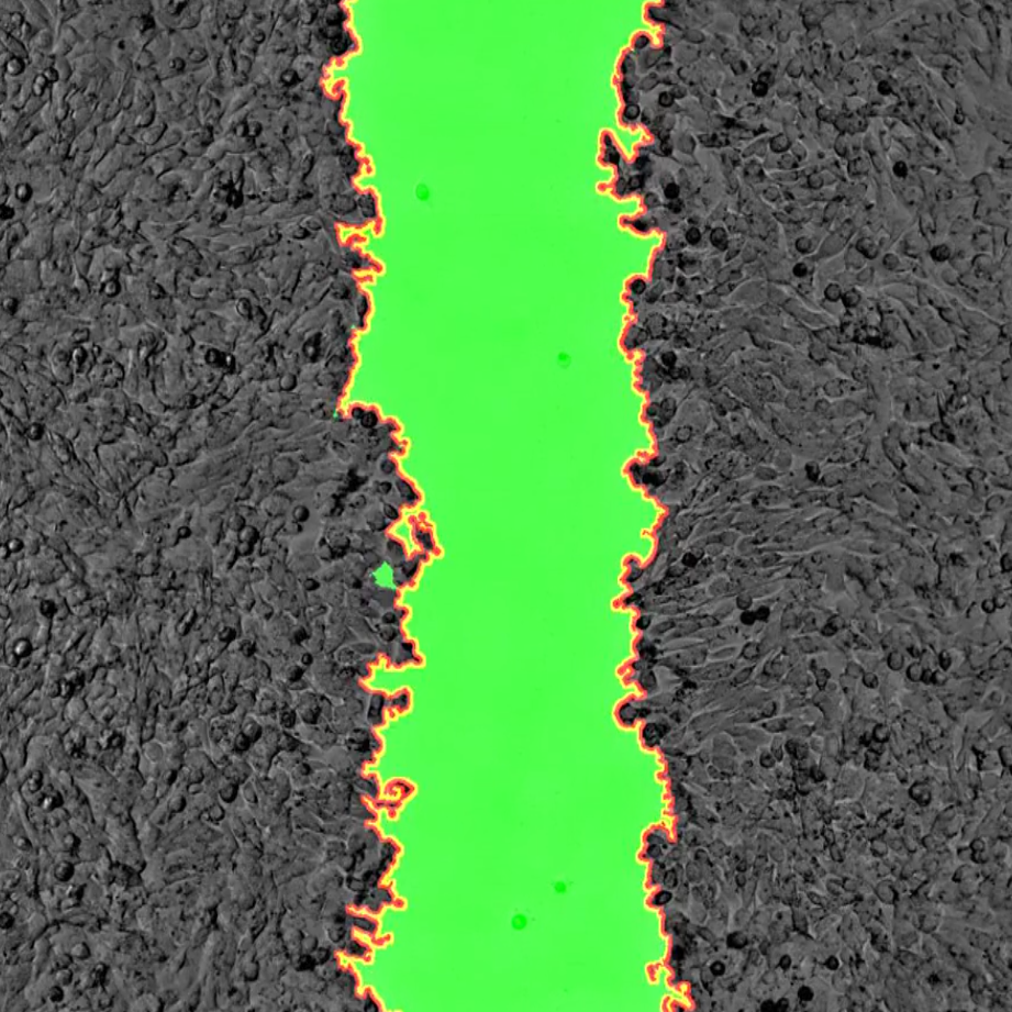
From the CCI website gallery. Data c/o Daimark Bennett
for movie
From the CCI website gallery. Data c/o Daimark Bennett
Applications: Batch Processing
Why batch process? File conversion, batch processing, scripting
Manual analysis (while sometimes necessary) can be laborious, error prone and not provide the provenance required. Batch processing allows the same processing to be run on multiple images.
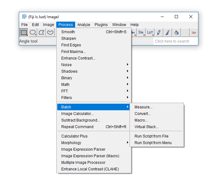
The built-in [Process > Batch] menu has lots of useful functions:
We'll use a subset of dataset BBBC008 from the Broad Bioimage Benchmark Collection
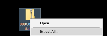
- Download the zip file from here to the desktop
- Unzip (right click and "Extract All") to end up with a folder on your desktop called
BBBC008_partial
- Make another folder on the desktop called
Output
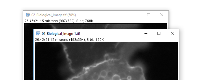
For simple file conversion, Convert is a very useful tool
- Run
[Process > Batch > Convert] - Set the Input directory to point to the downloaded files and the Output to the Output folder
- Set the output format to PNG
- Scale the images to 50% (put 0.5 in the box)
- Hit Convert then check the output folder
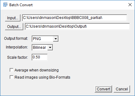
- If you're using proprietary formats check the "Read Using Bio-Formats" box (although this is slower)
For slightly more complex manipulations try using the Macro interface
- Run
[Process > Batch > Macro] - Set the Input directory to point to the downloaded files and the Output to the Output folder
- Set the output format to PNG
- From the dropdown box, select
Scaleand the macro box will populate - Change the scale fraction to 0.5 and add the line
run("Red"); - Hit Process then check the output folder
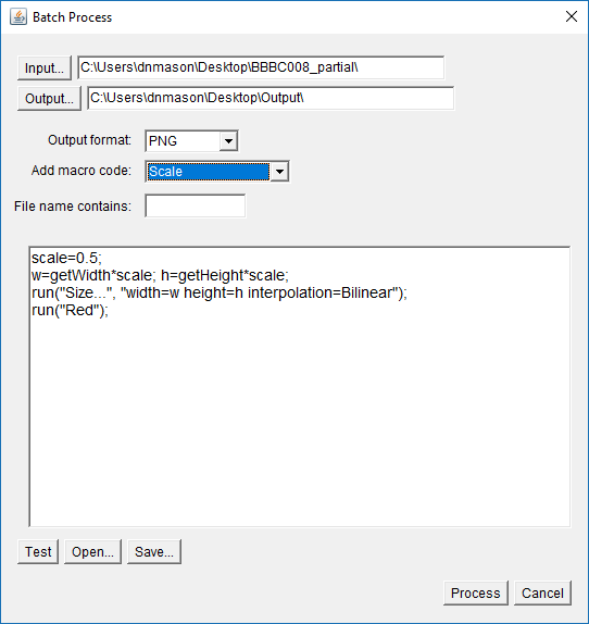
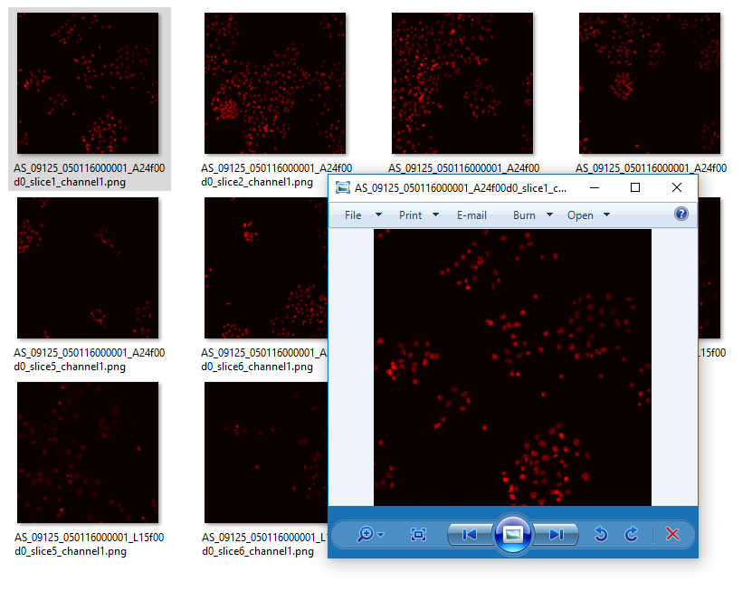
You should see an output folder containing small red-coloured nuclei
But how to figure out the commands?
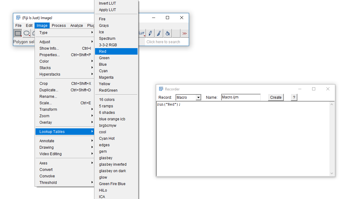
The macro recorder will record most plugins and commands from the menu. Run [Plugins > Macros > Record] then run a command
Pop quiz!
- Answers in the next slide - DON'T PEEK UNLESS YOU'RE STUCK :)
Basic test
//-- Calibrate
run("Properties...", "unit=um pixel_width=0.1 pixel_height=0.1");
//-- Add the scale bar
run("RGB Color");
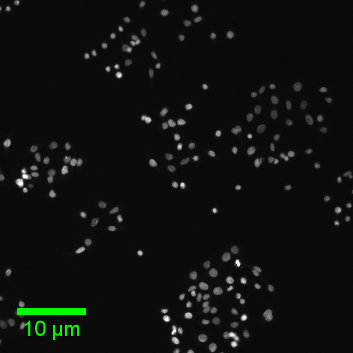
run("Scale Bar...", "width=10 height=10 font=30 color=Green background=None location=[Lower Left]");
Advanced test
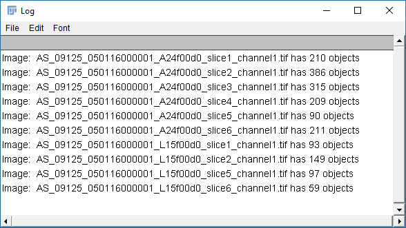
//-- [BONUS 2] Estimate and print the counts
run("Find Maxima...", "noise=10 output=[Point Selection]");
getSelectionCoordinates(xPos,yPos);
print("Image: "+getTitle()+" has "+xPos.length+" objects");
run("Select None");
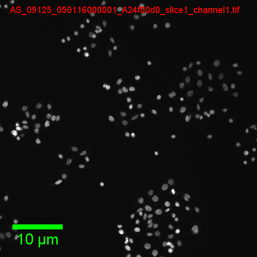
//-- [BONUS 1] Add the title
run("RGB Color");
setFont("SansSerif", 18, "antialiased");
setColor("red");
drawString(getTitle(), 20, 30);
//-- Calibrate
run("Properties...", "unit=um pixel_width=0.1 pixel_height=0.1");
//-- Add the scale bar
run("RGB Color");
run("Scale Bar...", "width=10 height=10 font=30 color=Green background=None location=[Lower Left]");
Scripting
A very brief foray into scripts
Scripting is useful for running the same process multiple times or having a record of how images were processed to get a particular output
Fiji supports many scripting languages including Java, Python, Scala, Ruby, Clojure and Groovy through the script editor which also recognises the macro language from the previous example (which we'll be using)
As an example, we're going to (manually) create a montage from a three channel image, then see what the script looks like
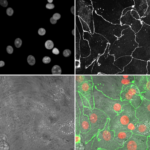
- Open
06-MultiChannel.tif - Open the macro recorder:
[Plugins > Macros > Record]
- (If opening via URL run
[Image > Hyperstacks > Stack to Hyperstack]) - Open the channels tool
[Image > Color > Channels Tool]and set the mode tograyscale - Run
[Image > Type > RGB color] - Rename this image to
channelswith[Image > Rename] - Select the original stack, and using the channels tool, set the mode to
composite - Run
[Image > Type > RGB color] - Rename this image to
mergewith[Image > Rename] - Close the original (it should be the only 8-bit image open (check the Info bar!)
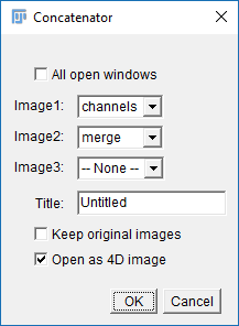
- Run
[Image > Stacks > Tools > Concatenate]and select Channels and merge in the two boxes (see right) - Run
[Image > Stacks > Make Montage]change the border width to 3 then hit OK
Got it? Have a look at the Macro Recorder and see if you can see the commands you ran
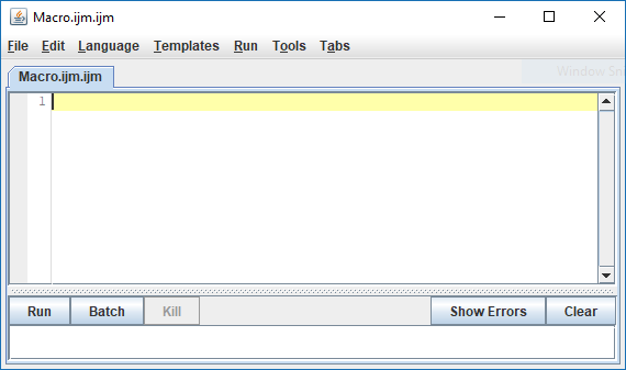
Open the script editor with [Plugins > New > Script] and copy in the following code:
//-- Record the filename
imageName=getTitle();
print("Processing: "+imageName);
//-- Display the stack in greyscale, create an RGB version, rename
Stack.setDisplayMode("grayscale");
run("RGB Color");
rename("channels");
//-- Select the original image
selectWindow(imageName);
//-- Display the stack in composite, create an RGB version, rename
Stack.setDisplayMode("composite");
run("RGB Color");
rename("merge");
//-- Close the original
close(imageName);
//-- Put the two RGB images together
run("Concatenate...", "  title=newStack open image1=channels image2=merge");
//-- Create a montage
run("Make Montage...", "columns=4 rows=1 scale=0.50 border=3");
//-- Close the stack (from concatenation)
close(newStack);
Open the file again and hit Run
Comments, variables, print, active window
This script operates on an open image but it's easily converted to a batch processing script using the built in templates:
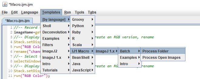
The full script is here. I added these lines at the top and bottom:
open(input + File.separator + file);saveAs("png", output + File.separator + replace(file, suffix, ".png"));
close("*");
If you're interested in a scripting workshop, let me know! We can put one together in the near future.
In the meantime:
Applications: Co-localisation
Use cases, some simple guidance, JaCoP
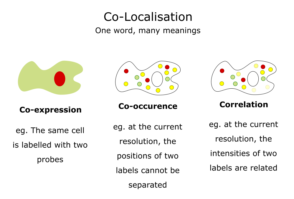
Adapted from a slide by Fabrice Cordelieres
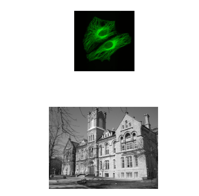
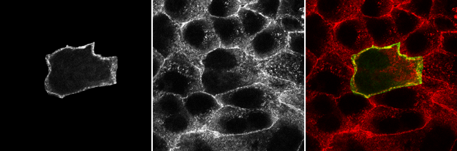
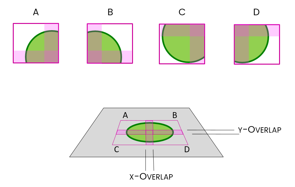
Colocalisation is highly dependent upon resolution! Example:
Same idea goes for cells. Keep in mind your imaging resolution!
We will walk through using JaCoP (Just Another CoLocalisation Plugin) to look at Pearson's and Manders' analysis
If you're doing colocalisation analysis at all, I highly recommend reading the companion paper https://doi.org/10.1111/j.1365-2818.2006.01706.x
Pearson's Correlation Coefficient
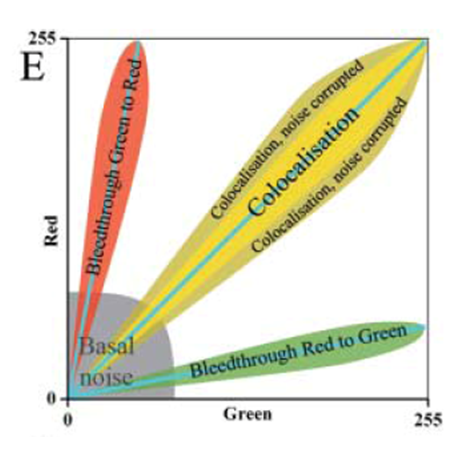
- For each pixel, plot the intensities of two channels in a scatter plot
- Ignore pixels with only one channel (IE intensity below BG)
- P value describes the goodness of fit (-1 to 1)
- 1 = perfect correlation
- 0 = no positive or negative correlation
- -1 = exclusion
Figure from https://doi.org/10.1111/j.1365-2818.2006.01706.x
- Download
JaCoP - Run
[Plugins > Install Plugin], point to the jar file - Restart Fiji
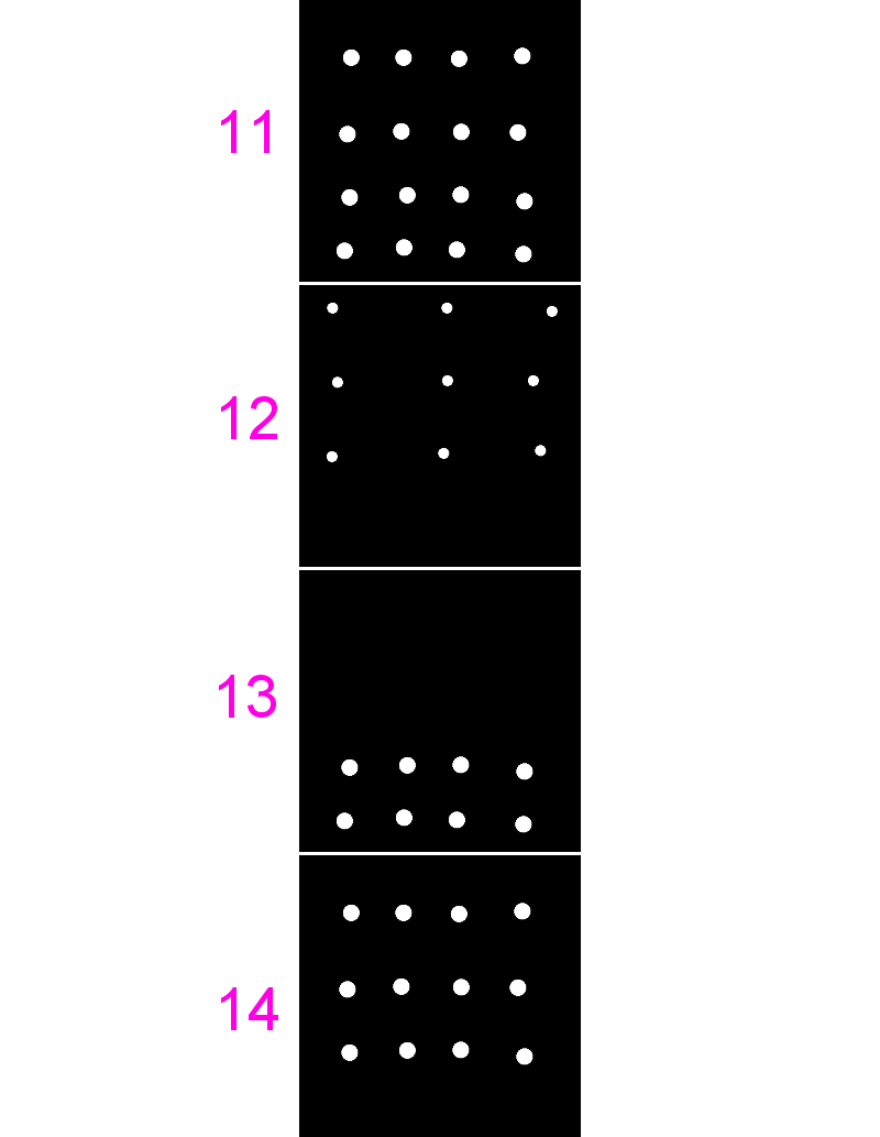
- Open
11-colocA.tifand12-colocB.tif - Run
[Plugins > JaCoP], uncheck everything except Pearsons, select the same image for both channels - Repeat for different combinations of these images and also
13and14
- Great for complete colocalisation
- Unsuitable if there is a lot of noise or partial colocalisation (see below)
- Midrange P-values (-0.5 to 0.5) do not allow reliable conclusions to be drawn
- Bleedthrough can be particularly problematic (as they will always correlate)
Manders' Overlap Coefficient
- Removes some of the intensity dependence of Pearson's and provides channel-specific overlap coefficients (M1 & M2)
- Values from 0 (no overlap) to 1 (complete overlap)
- Defined as "the ratio of the summed intensities of pixels from one channel for which the intensity in the second channel is above zero to the total intensity in the first channel"
- Use the same images from last time (
11,12,13and14) - Run
[Plugins > JaCoP], check both Pearsons and Manders - Run for different combinations of these images
- Note the differences in coefficients especially in images 13 and 14
- [BONUS] add some noise
[Process > Noise > Add Noise]or blur your images[Process > Filters > Gaussian Blur]and see how that affects the coefficients
Applications: Tracking
Correlating spatial and temporal phenomena, Feature detection, linkage, gotchas
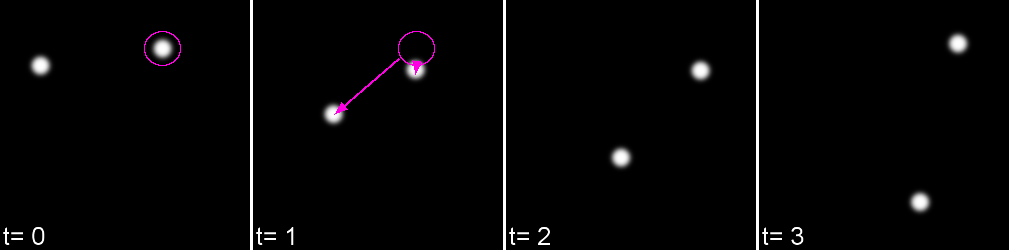
Life exists in the fourth dimension. Tracking allows you to correlate spatial and temporal properties.
Most partcles look the same! Without any way to identify them, tracking is probabilistic.
Tracking has two parts: Feature Identification and Feature Linking
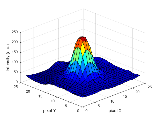
For every frame, features are detected, typically using a Gaussian-based method (eg. Laplacian of Gaussian: LoG)
Spots can be localised to sub-pixel resolution!
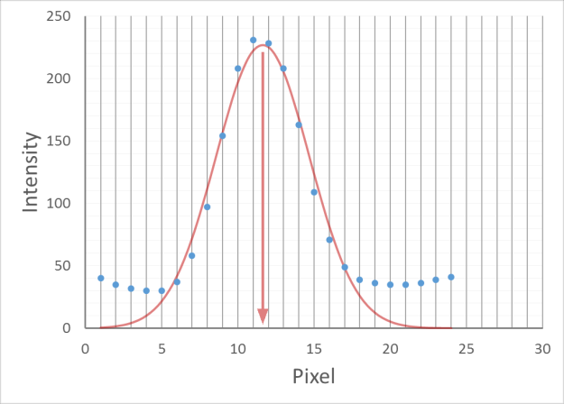
Without sub-pixel localisation, the precision of detection is limited to whole pixel values.
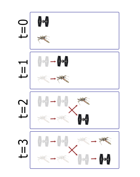
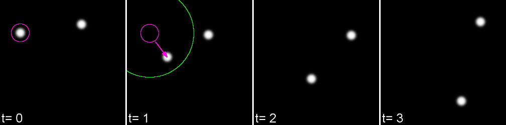
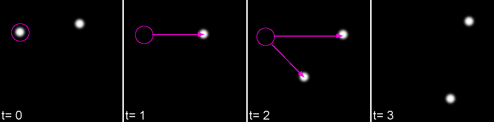
Feature linkage
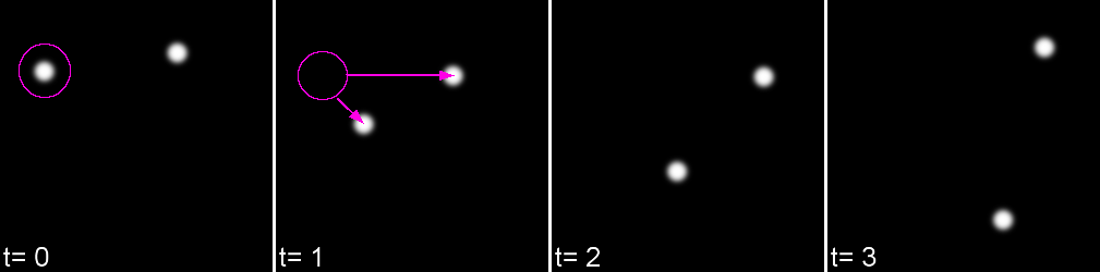
For each feature, all possible links in the next frame are calculated. This includes the spot disappearing completely.
A 'cost matrix' is formed to compare the 'cost' of each linkage. This is globally optimised to calculate the lowest cost for all linkages.
In the simplest form, a cost matrix will usually consider distance. Many other parameters can be used such as:
- Intensity
- Shape
- Quality of fit
- Speed
- Motion type
Which can allow for a more accurate linkage especially in crowded or low S/N environments
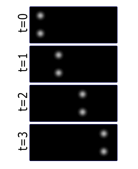
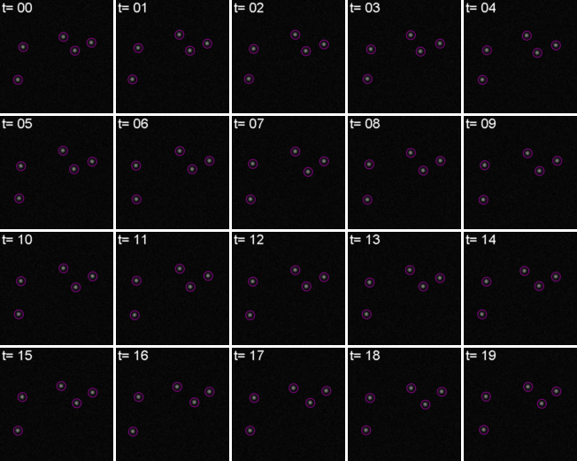
Open 10-tracks.tif
Hit the arrow to play the movie. Right Click on the arrow to set playback speed
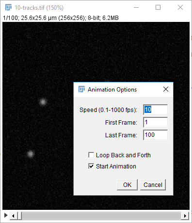
If you're interested in how the dataset was made see this snippet
Run [Plugins > Tracking > Trackmate]
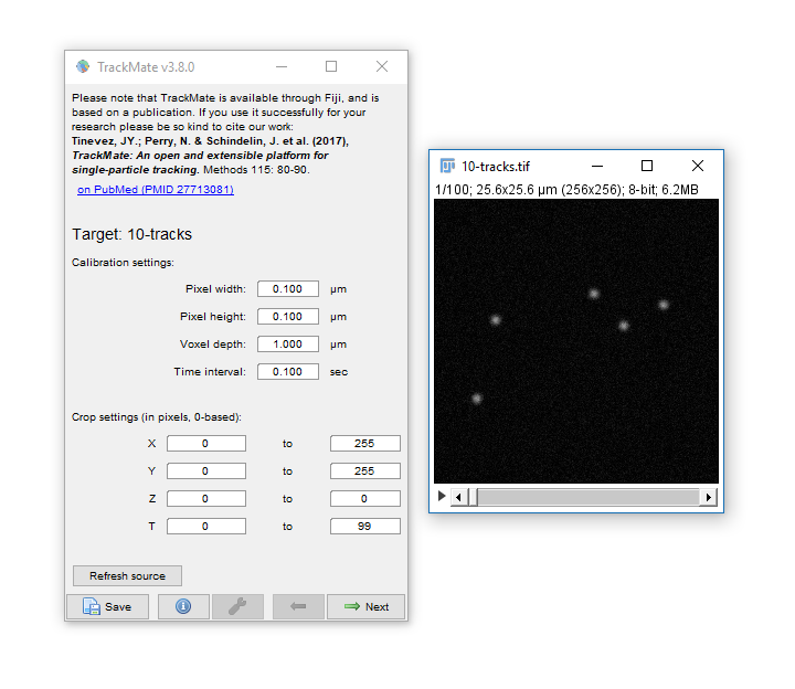
- Trackmate guides you through tracking using the Next and Prev buttons
- The first dialog lets you select a subset (in space and time) to process. This is handy on large datasets when you want to calculate parameters before processing the whole dataset
- Hit Next, keep the default (LoG) detector then hit Next again to move onto Feature detection.
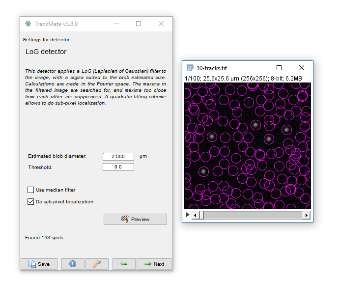
- Enter a Blob Diameter of 2 (note the scaled units)
- Hit preview. Without any threshold, all the background noise is detected as features
- Add a threshold of 0.1 and hit Preview again.
Generally your aim should be to provide the minimum threshold that removes all noise. Slide the navigation bar, then hit Preview to check out a few other timepoints.
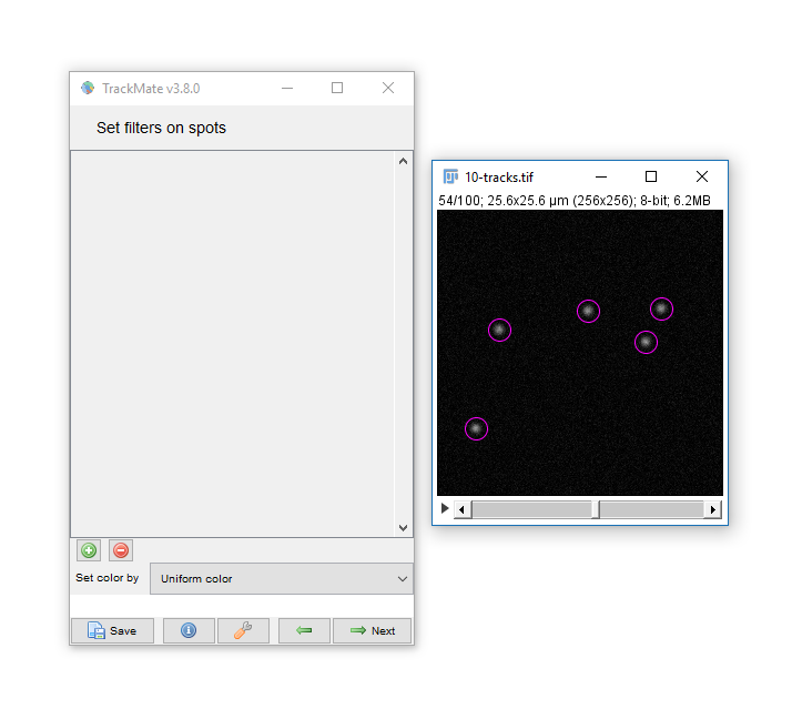
Hit next, accepting defaults until you reach 'Set Filters on Spots'
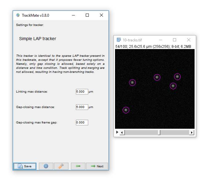
- Hit next, accepting defaults until you reach 'Settings for Simple LAP tracker'
- Keep the defaults and hit Next
- You have tracks!
Linking Max Distance Sets a 'search radius' for linkage
Gap-closing Max Frame Gap Allows linkages to be found in non-adjacent frames
Gap-closing Max Distance Limits search radius in non-adjacent frames
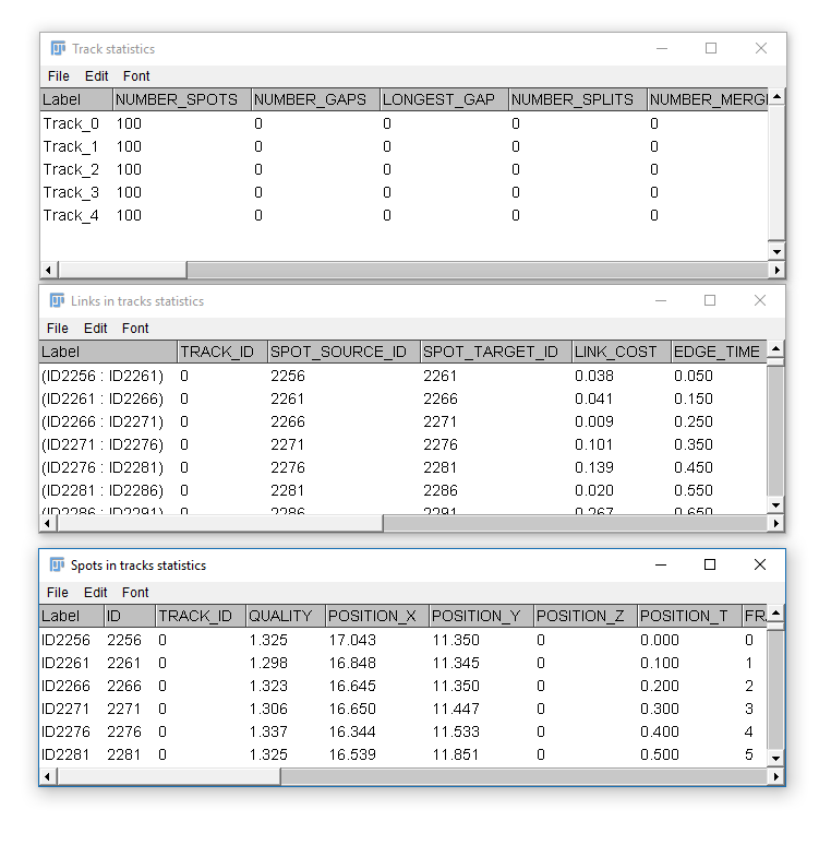
Common outputs from Trackmate: (1) Tracking data
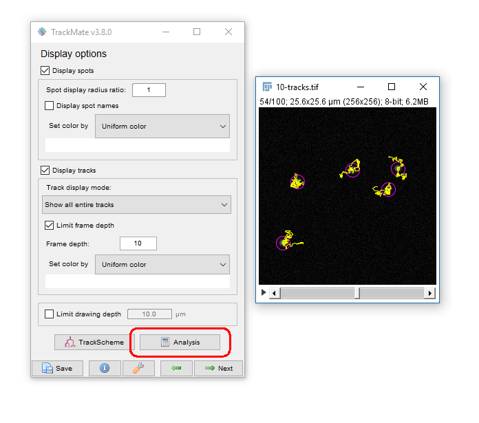
Common outputs from Trackmate: (2) Movies!
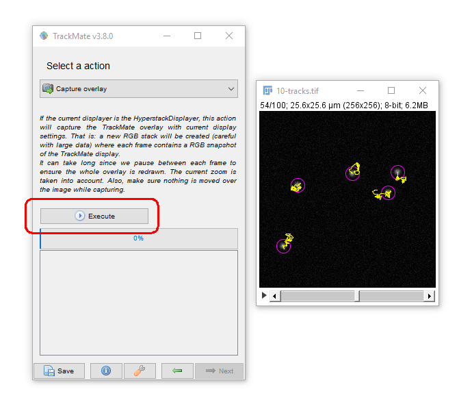
You may have to adjust the display options to get the tracks drawing the way you want (try "Local Backwards")
While simple, Tracking is not to be taken on lightly!
- For the best results make sure the inter-particle distance is greater than the frame-to-frame movement. If not, try to increase resolution (more pixels) or decrease interval (more frames)
- The search radius increases processing time with HUGE datasets but in most case, has little effect on processing time. Remember that closer particles will still be linked preferably if possible.
- Keep it simple! Unless you have problems with noise, blinking, focal shifts and similar, do not introduce gap closing as this may lead to false-linkages
- 'Simple LAP tracker' does not include merge/spliting events, however Trackmate ships with the more complex 'LAP Tracker' which can handle merge/splitting events (but keep in mind your system!)
- Quality control! Look at your output carefully and make sure you're not getting 'jumps' where one particle is linked to another incorrectly
Applications: Stitching
Resolution vs field size, stitching, using overlaps, issues and bugs
Increasing resolution (via higher NA lenses) almost always leads to a reduced field
Often you will want both!
We can achieve this with tile scanning (IE. imaging multiple adjacent fields)
Stitching is the method used to put them back together again
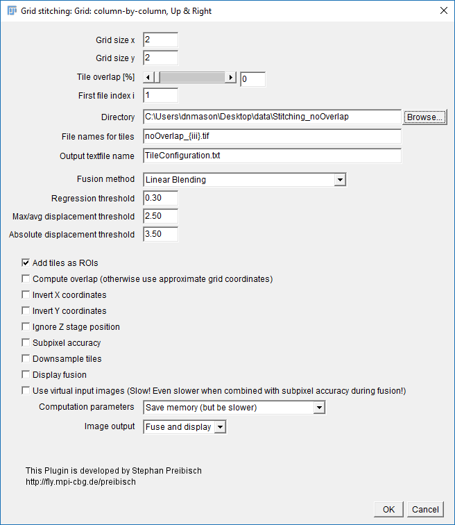
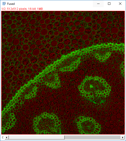
Images acquired as adjacent frames (zero overlap)
- Open
Stitching_noOverlap.zip. Unzip to the desktop. - Run
[Plugins > Stitching > Grid/Collection Stitching] - Select: Column by Column | Up & Right
- Settings:
- Grid Size: 2x2
- Tile Overlap: 0
- Directory: {path to your folder}
- File Names: replace the numbers with
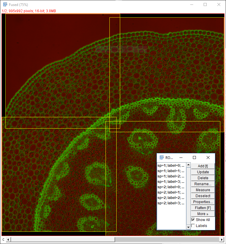
{i}zero pad with morei- noOverlap_{iii}.tif - Uncheck all the options [OPTIONAL] Check add as ROI
- Hit OK (accept fast fusion)
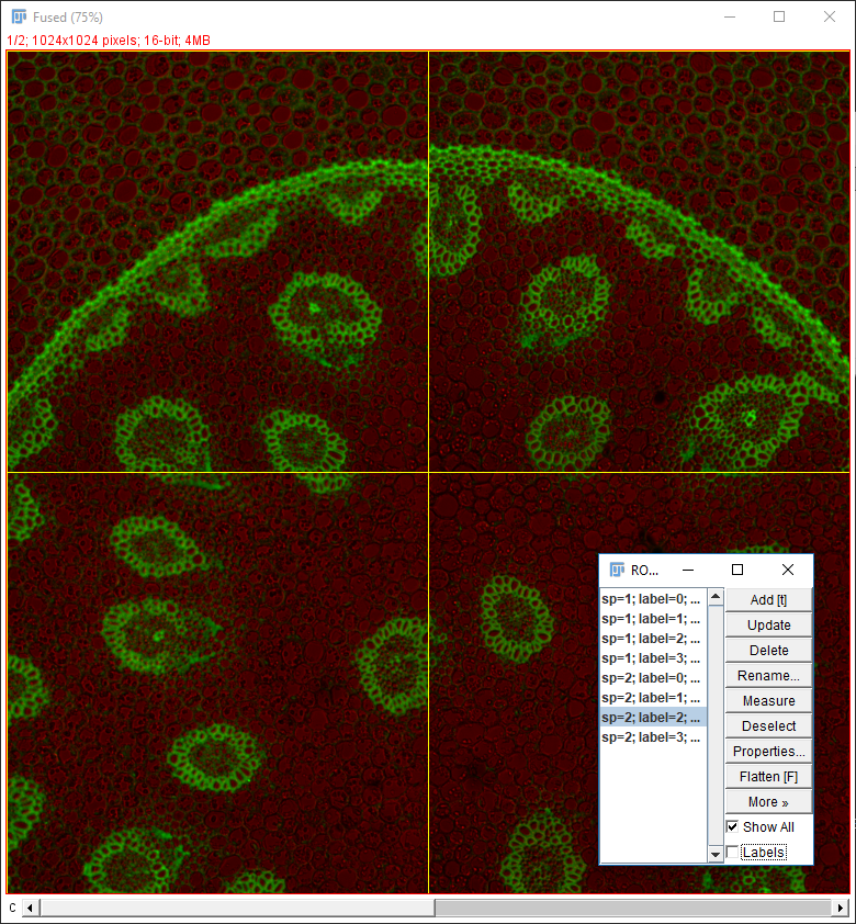
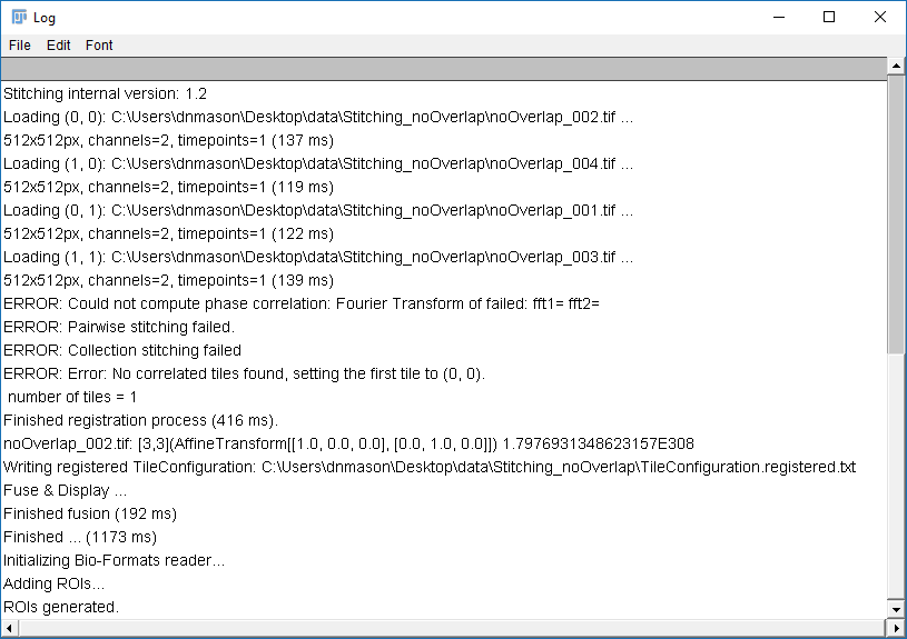
Why do the images not line up?
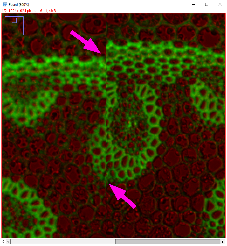
Run [Plugins > Stitching > Grid/Collection Stitching] again
Check the settings are as before but add "compute overlap" and hit OK
- Open
Stitching_Overlap.zip. Unzip to the desktop. - Run
[Plugins > Stitching > Grid/Collection Stitching]again - Change the directory, filename and overlap.
- Hit OK
Two things to remember when using Grid/Collection Stitching:
- Default (R,G,B) LUTs are used after stitching ()
- All calibration information is stripped ()
- Stitching will have a harder time with sparse features or uneven illumination (example here)
The most important point is to know your data!
- Grid layout (dimensions and order!)
- Overlap
- Calibration
Thank you for your attention!
We will send you a survey for feedback; please take 2 minutes to answer, it helps us a lot!